Nullspace EM Tutorial Series: Antenna Array Design

This is part 2 of a 6-part tutorial series hosted by experienced antenna engineer Katerina Galitskaya who is documenting her experience learning Nullspace as a new user. Over six tutorials she will progress from simulating a single bow-tie antenna to building full arrays and exploring beamforming techniques, sharing direct comparisons to other full-wave 3D EM simulation tools.

The full video version of this tutorial is available to watch on YouTube.

Problem Statement

This tutorial presents the modeling, simulation, and post-processing of a 4-element antenna array based on the over-the-ground bow-tie antenna created in the previous tutorial. Antenna arrays are employed in various applications where high gain and controlled beam patterns are required. The final 3D geometry is shown in Figure 1.

Fig. 1 4-element antenna array

Model setup

Preparation: Use the single bow-tie element model from the first tutorial.

Units: CAD model is defined in millimeters, converted to meters during simulation.

Frequency sweep: 0.5–1.5 GHz.

Radiation data: Dense far‑field grid (2-degree step in theta and phi).

Extracted metrics: Return loss, input impedance, boresight gain, gain vs. frequency, 2D radiation cuts, and 3D radiation pattern.

CAD Model and Meshing

Begin by opening Prep and setting your working directory to a folder where you plan to complete this example.

Complete the modeling of a single antenna element as described in detail in the first tutorial.

#{inner_width=1.7}

#{outer_width=30}

#{leng=42}

#{port=1.7}

#{subH=0.767}

#{subW=140}

brick x {subW} y {subW} z {subH}

volume 1 rename "substrate"

move Volume substrate z {-subH/2} include_merged 

create vertex {-port/2} {-port/2} 0 

#{v1 = Id("vertex")}

create vertex {port/2} {-port/2} 0

create vertex {port/2} {0} {port/4}

create vertex {-port/2} {0} {port/4}

create surface vertex {v1} to {v1+3}

#{port_pos = Id("surface")}

surface {port_pos} copy reflect y 

#{port_neg = Id("surface")}

create curve location {-outer_width/2} {port/2+leng} 0 location {outer_width/2} {port/2+leng} 0

#{c1 = Id("curve")}

create curve location {-outer_width/2} {port/2+leng} 0 location {-inner_width/2} {port/2} 0

create curve location {outer_width/2} {port/2+leng} 0 location {inner_width/2} {port/2} 0

create curve location {-inner_width/2} {port/2} 0 location {inner_width/2} {port/2} 0

create surface curve {c1} to {c1+3}

#{dipole_top = Id("surface")}

surface {dipole_top} copy reflect y nomesh 

#{dipole_bot = Id("surface")}

project surface {port_pos} {port_neg} onto surface 1 imprint

project surface {port_pos} {port_neg} {dipole_top} {dipole_bot} onto surface 2 imprint

create surface rectangle width 300 zplane 

#{GND = Id("surface")}

#{gnd_H=70}

move Volume 6 z {-gnd_H} include_merged preview 

move Volume 6 z {-gnd_H} include_merged

Now, replicate the bow-tie element to form a 4-element array. Ensure that spacing between elements lies within the range λ > D > λ/2 to prevent grating lobes. 

Volume 1 2 3 4 5 6 copy move x 0 y 300 z 0 repeat 3 group_results ###copying/moving the element along Y axis

rotate Volume all angle 90 about Y include_merged preview 

rotate Volume all angle 90 about Y include_merged 

imprint all

merge all

Materials & Voltage Sources

Use the provided Python script material.py to define a material library. Only FR-4 and PEC are used in this example. Open the Nullspace EM environment and load the material.py file before assigning materials.

from nsem import *

ml=MaterialLibrary()

ml.add_material(Material('FR-4', 'green', MaterialProperty('constant',real=4.4, losstan=0.02), MaterialProperty('constant',real=1.0, imag=0.0)))

ml.save('materials')

Assign materials and define four voltage sources. Ensure consistent assignment of positive and negative terminals across all ports.

nsem load material library 'materials.h5'

nsem assign volume substrate material 'FR-4' ###the original substrate

nsem assign volume 7 13 19 material 'FR-4' ###the 3 copies

nsem assign surface {dipole_top} {dipole_bot} material 'PEC' ###the original antenna

nsem assign surface 34 35 36 51 52 53 68 69 70 material 'PEC' ###the 3 copies

nsem voltage source 'port_001' pos surface {port_pos} neg surface {port_neg} impedance 50

nsem voltage source 'port_002' pos surface 32 neg surface 33 impedance 50

nsem voltage source 'port_003' pos surface 49 neg surface 50 impedance 50

nsem voltage source 'port_004' pos surface 66 neg surface 67 impedance 50

nsem assign surface {GND} material 'PEC'

Meshing

Group the two port surfaces for easier reference and assign appropriate mesh sizes.

group 'feed' add surface {port_pos} {port_neg} 32 33 49 50 66 67

Assign the port mesh keeping in mind that the curve common to the voltage source surfaces for each feed should have a single mesh edge.

curve common_to surface in feed interval 1

mesh surface in feed

Apply a denser mesh to the antenna arms for improved accuracy. Assign mesh to the rest of the model normally.

surface all scheme pave

#{mesh=0.3/1.5*1000/10}

group 'feed' add surface {port_pos} {port_neg} 32 33 49 50 66 67

curve common_to surface in feed interval 1

mesh surface in feed

surface {dipole_top} {dipole_bot} 34 35 51 52 68 69 size {mesh/4}

mesh surface {dipole_top} {dipole_bot} 34 35 51 52 68 69

surface 14 16 17 18 size {mesh/4}

mesh surface 14 16 17 18

surface {GND} 36 53 70 size {mesh/1.5}

mesh surface {GND} 36 53 70

surface not is_meshed in volume 1 7 13 19 size {mesh/4}

mesh surface not is_meshed in volume 1 7 13 19

block 1 surface all

save cub5 "Bowtie_array.cub5" overwrite journal

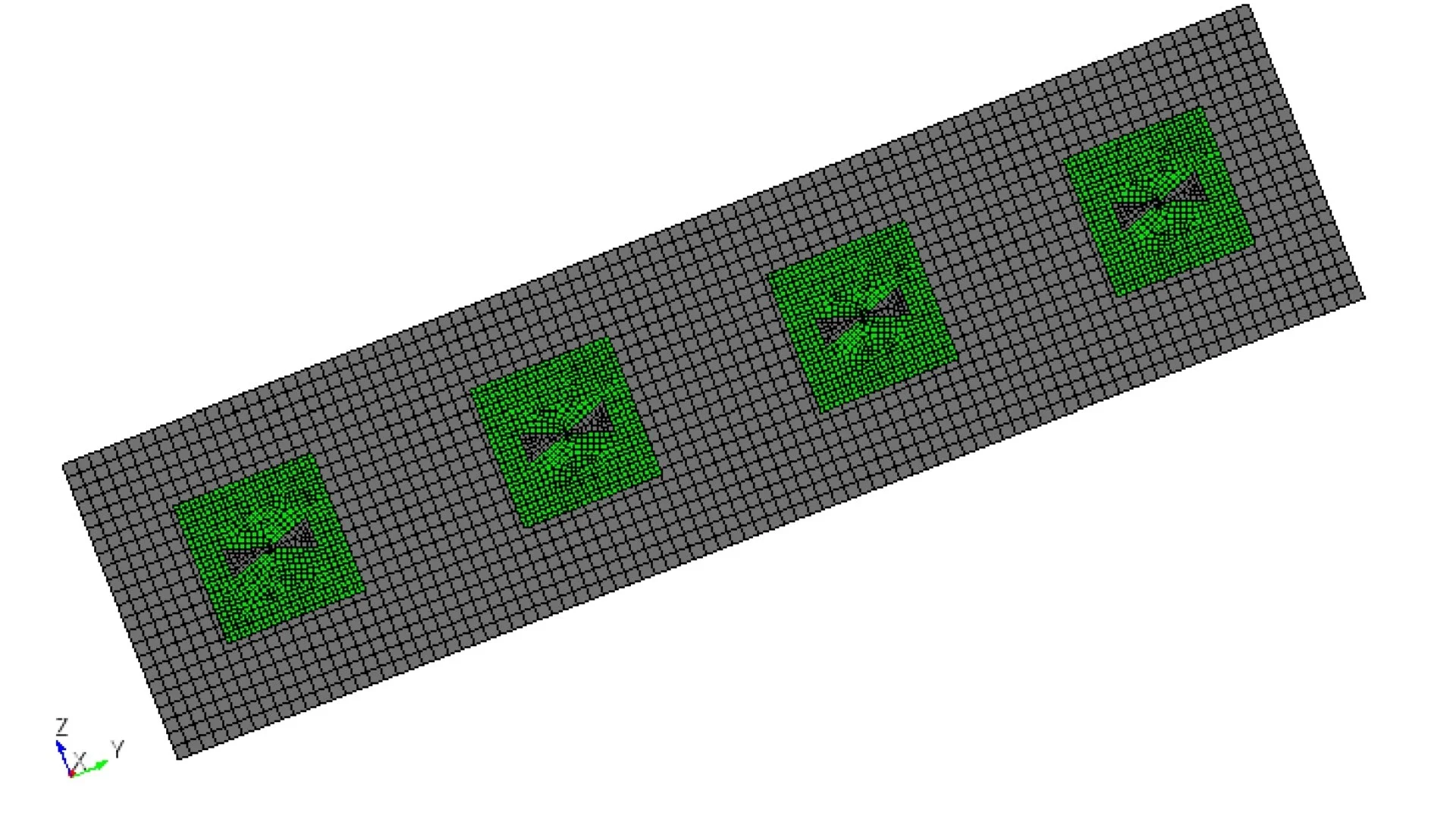
Fig.2 Model with the final mesh.

Simulation Setup

Create a simulation.py file to configure the simulation parameters.

from nsem import *

import numpy as np

config = 'Bowtie_array'

model = Configuration(f'{config}_sim') #configure simulation name

model.set_cub5_filename(f'{config}.cub5') #load the mesh file

model.set_order(1) #set basis order, default is 1

model.set_model_scale(0.001) #convertion to mm

model.set_frequencies(freq_beg=0.5, freq_end=1.5) #set frequency sweep from 0.5 to 1.5 GHz

model.save()

report = Report(f'{config}_report', f'{config}_sim') #create a report object

report.set_frequencies(np.linspace(0.5, 1.5, 11))

step = 2 #set the step for theta and phi angles

theta_scan = np.linspace(0, 180, int(180/step+1)) #theta angles from 0 to 180 degrees

phi_scan = np.linspace(0, 360, int(360/step)) #phi angles from 0 to 360 degrees

report.request_far_fields_grid(theta_scan, phi_scan) #request far-field data

report.save() #save the report configuration

model.run() #run the simulation

report.run() #run the report generation

Post-Processing

Create postprocessing.py to extract simulation data and visualize results.

In antenna array simulations, active S-parameters are more relevant than traditional return loss, as they also account for coupling between elements.

The new variable w defines the amplitude and phase excitation for each element. Here we use equal amplitude and zero phase shift.

import matplotlib.pyplot as plt

import numpy as np

from nsem.postprocessing import *

config = 'Bowtie_array'

post = PostProcess(f'{config}_sim') # create a post-processing object for the simulation

freq = post.get_frequencies() # get the frequencies from the report

freq = np.linspace(np.min(freq), np.max(freq), 501) # create a frequency array for evaluation

sparam = post.get_s_parameters(freq_evaluate=freq) # get the S-parameters

rl = dB20(np.squeeze(sparam[0, 0, :])) # convert S-parameters to dB scale

w = [1.0, 1.0, 1.0, 1.0] #equal excitation of each port

active_s = post.get_active_s_parameters(freq_evaluate=freq,weights=w) #get active s-parameters with defined weights

active_s11 = dB20(np.abs(np.mean(active_s, axis=0))) #get the combined active parameters for all 4 ports

#plots

fig = plt.figure(figsize=(18, 6))

ax1 = plt.subplot(1, 3, 1)

ax2 = plt.subplot(1, 3, 2)

ax3 = plt.subplot(1, 3, 3, polar=True)

#active S-parameters

ax1.plot(freq, active_s11, label='active S11 combined', color='blue')

ax1.set_xlabel('Frequency (GHz)')

ax1.set_ylabel('active S11 (dB)')

ax1.set_title('Active S-parameters')

ax1.grid(True)

ax1.legend()

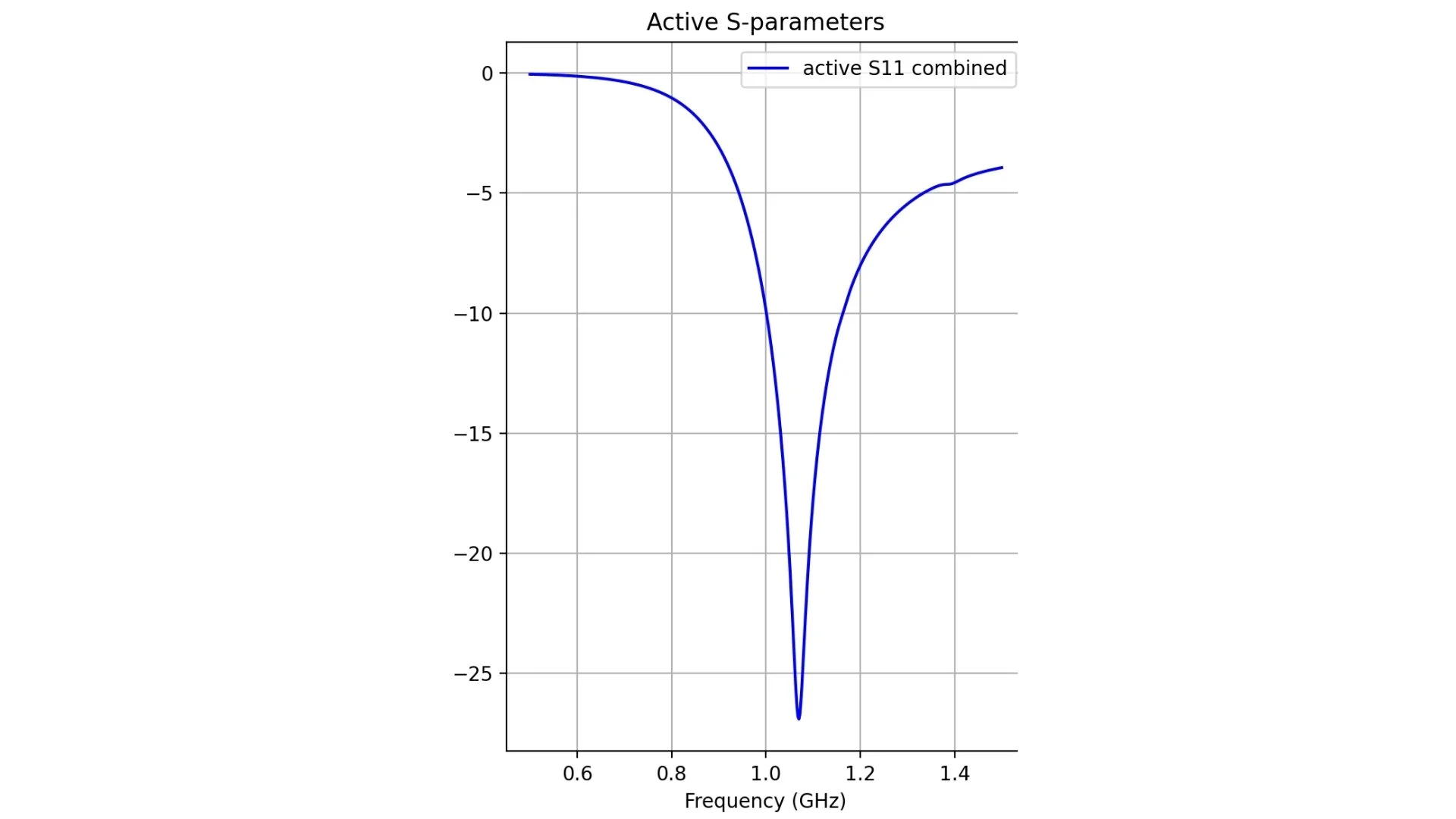
Fig. 3 Combined active S11

post = PostProcess(f'{config}_report') # create a post-processing object for the report

freq = post.get_frequencies()

theta = post.get_obs_theta()

phi = post.get_obs_phi()

gain = post.get_gain('spherical',weights=w) #get gain with specified amplitude/phase distribution

theta_idx,_ = post.get_nearest(theta, 0.0)

phi0_idx,_ = post.get_nearest(phi, 0.0)

phi90_idx,_ = post.get_nearest(phi, 90.0)

theta90_idx,_ = post.get_nearest(theta, 90.0)

theta0_idx,_ = post.get_nearest(theta, 0.0)

freq_idx,_ = post.get_nearest(freq, 1.0)

gain_0 = gain[phi0_idx, theta90_idx, 0, freq_idx, 1]

print(f"Boresight gain (dBi): {gain_0:.2f}")

gain_copol_phi0 = gain[phi0_idx, :, 0, freq_idx,1]

gain_copol_phi90 = gain[phi90_idx, :, 0, freq_idx, 0]

gain_xpol_phi0 = gain[phi0_idx, :, 0, freq_idx, 0]

gain_xpol_phi90 = gain[phi90_idx, :, 0, freq_idx, 1]

gain_copol_theta90 = gain[:, theta90_idx, 0, freq_idx, 1]

gain_xpol_theta90 = gain[:, theta90_idx, 0, freq_idx, 0]

# --- Gain vs frequency ---

gain_max = np.squeeze(gain[phi0_idx, theta90_idx, 0, :, 1])

ax2.plot(freq, gain_max, label='Gain', color='blue')

ax2.set_xlabel('Frequency (GHz)')

ax2.set_ylabel('Gain (dBi)')

ax2.set_title('Boresight Gain vs Frequency')

ax2.grid(True)

ax2.legend()

Fig. 4 Boresight gain over frequency

# Elevation cut

ax3.plot(np.deg2rad(phi), gain_copol_theta90, label=f'Co-pol theta=90°', color='green')

ax3.set_xlabel('phi (deg)')

ax3.set_ylabel('Gain (dBi)')

ax3.set_title('Elevation Cuts')

ax3.grid(True)

ax3.legend()

fig.tight_layout()

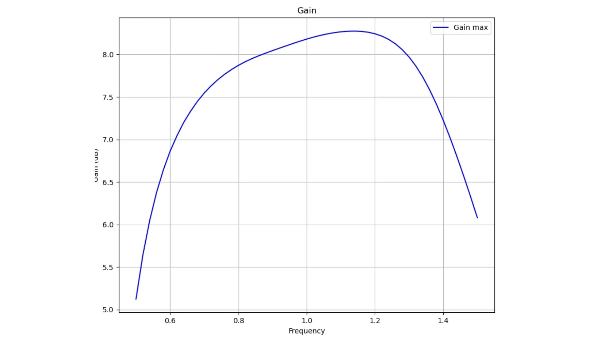
Fig. 6 Boresight gain over frequency

#pattern cut

ax4.plot(np.deg2rad(phi), gain_copol_theta90, label='Theta 90 copol', color='blue')

ax4.set_xlabel('Phi (deg)')

ax4.set_ylabel('Gain (dB)')

ax4.set_ylim([-30, 10])

ax4.grid(True)

ax4.legend()

fig.tight_layout()

fig.delaxes(ax6)  

fig.delaxes(ax5)  

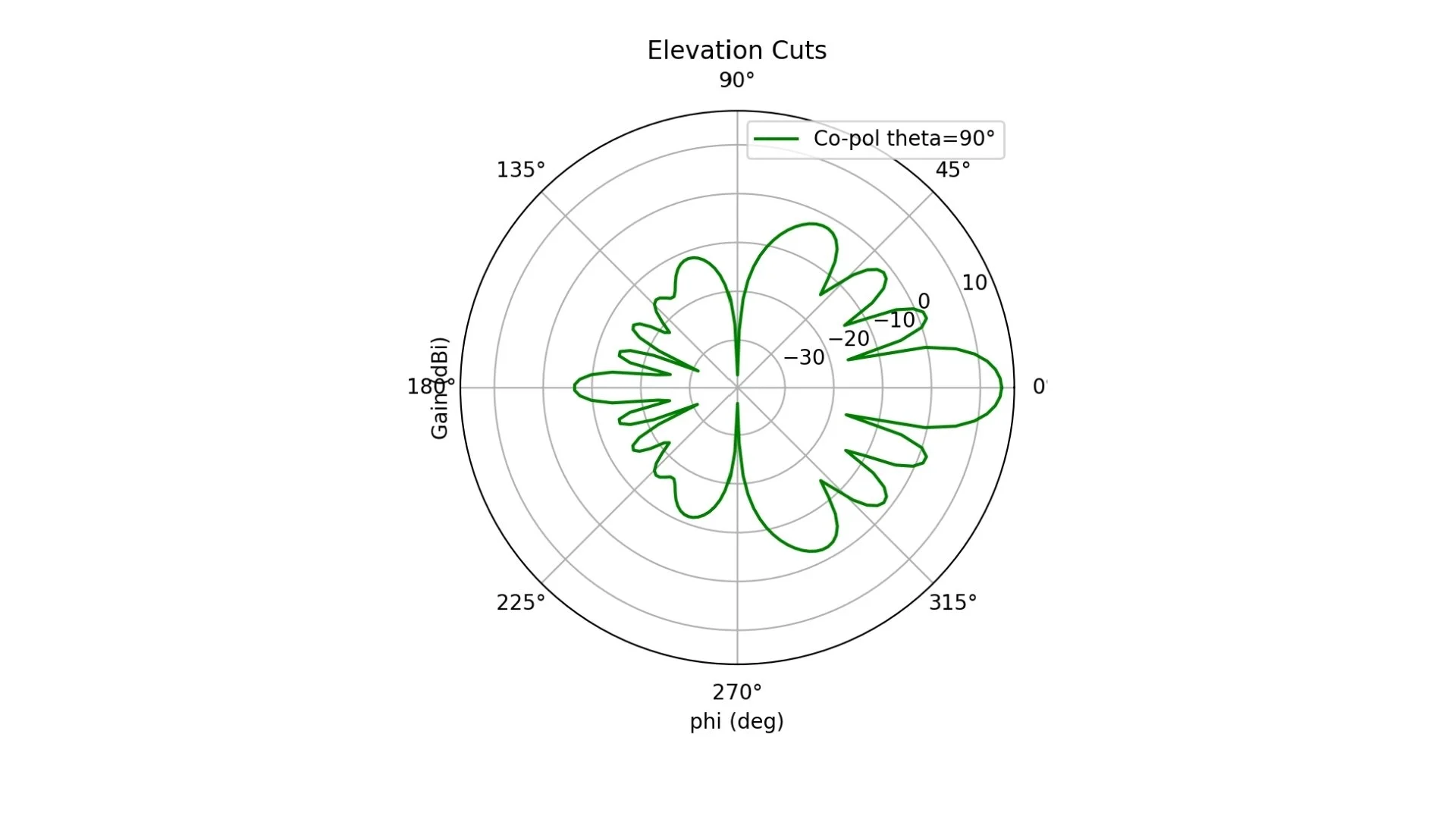
Fig. 5 Gain plot along phi, theta = 90

#3D radiation pattern

fig3d,ax3d = post.plotPolar3D(gain[:,:,0,freq_idx,1], -20.0,20.0)

fig3d.show()

plt.show()

Fig. 6 3D gain pattern