Nullspace EM Tutorial Series: Phased Array Beamforming Tutorial

This is part 3 of a 6-part tutorial series hosted by experienced antenna engineer Katerina Galitskaya who is documenting her experience learning Nullspace as a new user. Over six tutorials she will progress from simulating a single bow-tie antenna to building full arrays and exploring beamforming techniques, sharing direct comparisons to other full-wave 3D EM simulation tools.

The full video version of this tutorial is available to watch on YouTube.

Problem Statement

This tutorial demonstrates the post-processing capabilities for beamforming using the 4-element antenna array created in the previous tutorial.

Beamforming is a technique in which an antenna array is used to "steer" or direct radio signals toward a specific direction, rather than broadcasting energy uniformly in all directions within a sector. By controlling the amplitude and phase of the signal emitted from each antenna element, the resulting transmitted wave can be focused constructively in a desired direction or suppressed destructively in others. This approach enables precise beam control and enhanced signal strength in the targeted region.

The 4-element antenna array model used here is similar to the one that was created in the previous tutorial and is shown in Fig. 1.

Fig. 1 4-element antenna array

Model setup

Units: CAD model is defined in millimeters, converted to meters during simulation.

Frequency sweep: 0.5–1.5 GHz.

Radiation data: Dense far‑field grid (2-degree step in theta and phi).

Extracted metrics: Active S-parameters, boresight gain, gain vs. frequency, 2D radiation cuts, and 3D radiation pattern.CAD Model and Meshing

Begin by opening Prep and setting your working directory to a folder where you plan to complete this example.

Complete the modeling of a single antenna element as described in detail in the first tutorial.

CAD Model and Meshing

Begin by opening Prep and setting your working directory to a folder where you plan to complete this example.

Model the 4-element antenna array as described in the previous tutorial. Material and port assignments, as well as meshing strategies, remain unchanged. To minimize the grating lobes the distance between elements in array is decreased and is now close to lambda/2.

#{inner_width=1.7}

#{outer_width=30}

#{leng=42}

#{port=1.7}

#{subH=0.767}

#{subW=140}

###substrate geometry

brick x {subW} y {subW} z {subH}

volume 1 rename "substrate"

move Volume substrate z {-subH/2} include_merged 

###ports geometry

create vertex {-port/2} {-port/2} 0 

#{v1 = Id("vertex")}

create vertex {port/2} {-port/2} 0

create vertex {port/2} {0} {port/4}

create vertex {-port/2} {0} {port/4}

create surface vertex {v1} to {v1+3}

#{port_pos = Id("surface")}

surface {port_pos} copy reflect y 

#{port_neg = Id("surface")}

###antenna geometry

create curve location {-outer_width/2} {port/2+leng} 0 location {outer_width/2} {port/2+leng} 0

#{c1 = Id("curve")}

create curve location {-outer_width/2} {port/2+leng} 0 location {-inner_width/2} {port/2} 0

create curve location {outer_width/2} {port/2+leng} 0 location {inner_width/2} {port/2} 0

create curve location {-inner_width/2} {port/2} 0 location {inner_width/2} {port/2} 0

create surface curve {c1} to {c1+3}

#{dipole_top = Id("surface")}

surface {dipole_top} copy reflect y nomesh 

#{dipole_bot = Id("surface")}

project surface {port_pos} {port_neg} onto surface 1 imprint

project surface {port_pos} {port_neg} {dipole_top} {dipole_bot} onto surface 2 imprint

###ground plane

create surface rectangle width 300 zplane 

#{GND = Id("surface")}

#{gnd_H=70}

move Volume 6 z {-gnd_H} include_merged preview 

move Volume 6 z {-gnd_H} include_merged 

###4-element array creation

Volume 1 2 3 4 5 6 copy move x 0 y 170 z 0 repeat 3 group_results 

unite surface {GND} 36 53 70 ### creating a single surface for a common ground plane

#{GND = Id("surface")} #changing GND ID to the common one

rotate Volume all angle 90 about Y include_merged preview 

rotate Volume all angle 90 about Y include_merged 

imprint all

merge all

###assigning materials and ports

nsem load material library 'materials.h5'

nsem assign volume substrate material 'FR-4'

nsem assign volume 7 13 19 material 'FR-4'

nsem assign surface {dipole_top} {dipole_bot} material 'PEC'

nsem assign surface 34 35 51 52 68 69 material 'PEC'

nsem voltage source 'port_001' pos surface {port_pos} neg surface {port_neg} impedance 50

nsem voltage source 'port_002' pos surface 32 neg surface 33 impedance 50

nsem voltage source 'port_003' pos surface 49 neg surface 50 impedance 50

nsem voltage source 'port_004' pos surface 66 neg surface 67 impedance 50

nsem assign surface {GND} material 'PEC'

###meshing

surface all scheme pave

#{mesh=0.3/1.5*1000/10}

###port meshing

group 'feed' add surface {port_pos} {port_neg} 32 33 49 50 66 67

curve common_to surface in feed interval 1

mesh surface in feed

###antenna meshing

surface {dipole_top} {dipole_bot} 34 35 51 52 68 69 size {mesh/4}

mesh surface {dipole_top} {dipole_bot} 34 35 51 52 68 69

surface 14 16 17 18 size {mesh/4}

mesh surface 14 16 17 18

###GND meshing

surface {GND} size {mesh/1.5}

mesh surface {GND} 

###substrate meshing

surface not is_meshed in volume 1 7 13 19 size {mesh/4}

mesh surface not is_meshed in volume 1 7 13 19

block 1 surface all

save cub5 "Beamforming.cub5" overwrite journal

Simulation Setup

Simulation setup is identical to the previous tutorial, with the only change in scanning step to allow better accuracy while beamforming. 

step = 1 #set the step for theta and phi angles 

theta_scan = np.linspace(0, 180, int(180/step+1)) #theta angles from 0 to 180 degrees

phi_scan = np.linspace(0, 360, int(360/step))

Post-Processing

Create postprocessing.py to extract simulation data and visualize beamforming effects.

Beamforming is performed by adjusting the amplitude and phase at each of the four elements. In this example, two scenarios are evaluated:

1. 10-degree tilt using equal amplitudes (1,1,1,1).

2. 10-degree tilt with side-lobe suppression using unequal amplitudes (0.5, 1, 1, 0.5).
   

import matplotlib.pyplot as plt

import numpy as np

from scipy.signal import find_peaks

from nsem.postprocessing import *

from scipy.interpolate import CubicSpline

#Function to find weight at scan angle

def maximize_pattern_at_scan(ff, th, ph, th_scan, ph_scan):

    th_idx, _ = post.get_nearest(th, th_scan)

    ph_idx, _ = post.get_nearest(ph, ph_scan)

    # Extract far fields at scan angle: shape becomes [N_VS, N_f, 2]

    ff_scan = ff[ph_idx, th_idx, :, :, :]

    # Conjugate match for maximum gain (per element, per frequency, per polarization)

    weights = np.conj(ff_scan)

    # Normalize weights by total power

    norm = np.sqrt(np.sum(np.abs(weights) ** 2, axis=0, keepdims=True))

    weights_normalized = weights / norm

    return weights_normalized[:, :, 0], weights_normalized[:, :, 1]  # co-pol, cross-pol

config = 'Beamforming'

post = PostProcess(f'{config}_sim')  # create a post-processing object for the simulation

freq = post.get_frequencies()  # get the frequencies

freq = np.linspace(np.min(freq), np.max(freq), 501)  # create a frequency array for evaluation

post_report = PostProcess(f'{config}_report')  # create a post-processing object for the report

freq_report = post_report.get_frequencies()

theta = post_report.get_obs_theta()

phi = post_report.get_obs_phi()

th_scan = 90.0

ph_scan = 10.0 #set up the scan angle

w_co, w_cx = maximize_pattern_at_scan(post_report.get_far_fields(), theta, phi, th_scan, ph_scan)

# amplitude/phase tapering

N = w_co.shape[0]

amps = np.array([1, 1, 1, 1], dtype=float)[:N]

w_co *= amps[:, None]

# active S-parameters with the new weights

active_s = post.get_active_s_parameters(freq_evaluate=freq_report, weights=w_co)

active_s11 = dB20(np.squeeze(active_s[0, :]))

active_s22 = dB20(np.squeeze(active_s[1, :]))

active_s33 = dB20(np.squeeze(active_s[2, :]))

active_s44 = dB20(np.squeeze(active_s[3, :]))

gain = post_report.get_gain('spherical', weights=w_co)  # get the gain

# plots

fig = plt.figure(figsize=(18, 6), clear=False)

ax1 = plt.subplot(1, 3, 1)

ax2 = plt.subplot(1, 3, 2)

ax3 = plt.subplot(1, 3, 3, polar=True)

ax1.plot(freq_report, active_s11, label='active S11', color='blue')

ax1.plot(freq_report, active_s22, label='active S22', color='orange')

ax1.plot(freq_report, active_s33, label='active S33', color='green')

ax1.plot(freq_report, active_s44, label='active S44', color='red')

ax1.set_xlabel('Frequency (GHz)')

ax1.set_ylabel('dB')

ax1.set_title('Active S-parameters')

ax1.grid(True)

ax1.legend()

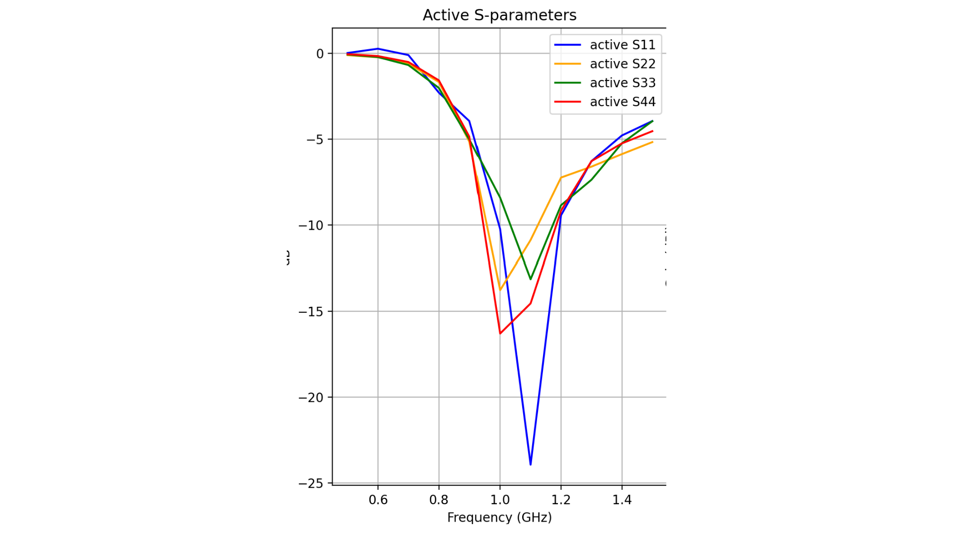
Fig. 2 Active S-parameters, [1, 1, 1, 1], 10-degree tilt

#calculating indexes 

theta_idx, theta_val = post.get_nearest(theta, 0.0)

phi0_idx = np.argmin(np.abs(phi - 0))

phi90_idx = np.argmin(np.abs(phi - 90))

theta90_idx = np.argmin(np.abs(theta - 90))

theta0_idx = np.argmin(np.abs(theta - 0))

freq_idx, freq_val = post.get_nearest(freq_report, 1)

# Max gain

gain_0 = gain[:, :, 0, freq_idx, 1]

max_gain = np.max(gain_0)

ph_idx_scan, ph_val_scan = post.get_nearest(phi, ph_scan)

th_idx_scan, th_val_scan = post.get_nearest(theta, th_scan)

#Printing max gain and tilt info

print(f'Max gain = {max_gain:.2f}dBi at Theta={th_scan:.1f}deg, Phi={ph_scan:.1f}deg')

print(f'Beam tilt = {ph_scan:.1f}deg')

# Find first upper side lobe and SLS

cut = gain_0[:, th_idx_scan]

main_idx = np.argmax(cut)

main_gain = cut[main_idx]

peaks, _ = find_peaks(cut)

side_lobe_candidates = [p for p in peaks if p > main_idx]  # Find all local peaks

if side_lobe_candidates:

    first_sidelobe_idx = side_lobe_candidates[0]

    first_sidelobe_gain = cut[first_sidelobe_idx]

    SLS = abs(first_sidelobe_gain - main_gain)

    print(f'First upper sidelobe = {first_sidelobe_gain:.1f}dBi (SLS = {SLS:.1f}dB)')

else:

    print('No upper sidelobe found')

# Cuts

gain_copol_phi0 = gain[phi0_idx, :, 0, freq_idx, 1]

gain_copol_phi90 = gain[phi90_idx, :, 0, freq_idx, 0]

gain_xpol_phi0 = gain[phi0_idx, :, 0, freq_idx, 0]

gain_xpol_phi90 = gain[phi90_idx, :, 0, freq_idx, 1]

gain_copol_theta90 = gain[:, theta90_idx, 0, freq_idx, 1]

gain_xpol_theta90 = gain[:, theta90_idx, 0, freq_idx, 0]

# Gain vs frequency

gain_max = np.squeeze(gain[ph_idx_scan, th_idx_scan, 0, :, 1])

#Gain plot interpolation

x = np.asarray(freq_report).ravel()

y = np.asarray(gain_max).ravel()

x_unique, idx = np.unique(x, return_index=True)

y_unique = y[idx]

cs = CubicSpline(x_unique, y_unique, bc_type='natural', extrapolate=False)

x_dense = np.linspace(x_unique[0], x_unique[-1], 501)

y_dense = cs(x_dense)

#Gain over frequency plot

ax2.plot(x_dense, y_dense, label=f'Gain at tilt {ph_scan:.1f}°', color='blue')

ax2.set_xlabel('Frequency (GHz)')

ax2.set_ylabel('Gain (dBi)')

ax2.set_title('Gain vs Frequency')

ax2.grid(True)

ax2.legend()

Fig. 3 Gain over frequency [1, 1, 1, 1], 10-degree tilt

# Cuts

ax3.plot(np.deg2rad(phi), gain_copol_theta90, label=f'Co-pol theta=90°', color='green')

ax3.set_xlabel('phi (deg)')

ax3.set_ylabel('Gain (dBi)')

ax3.set_title('Elevation Cuts')

ax3.grid(True)

ax3.legend()

fig.tight_layout()

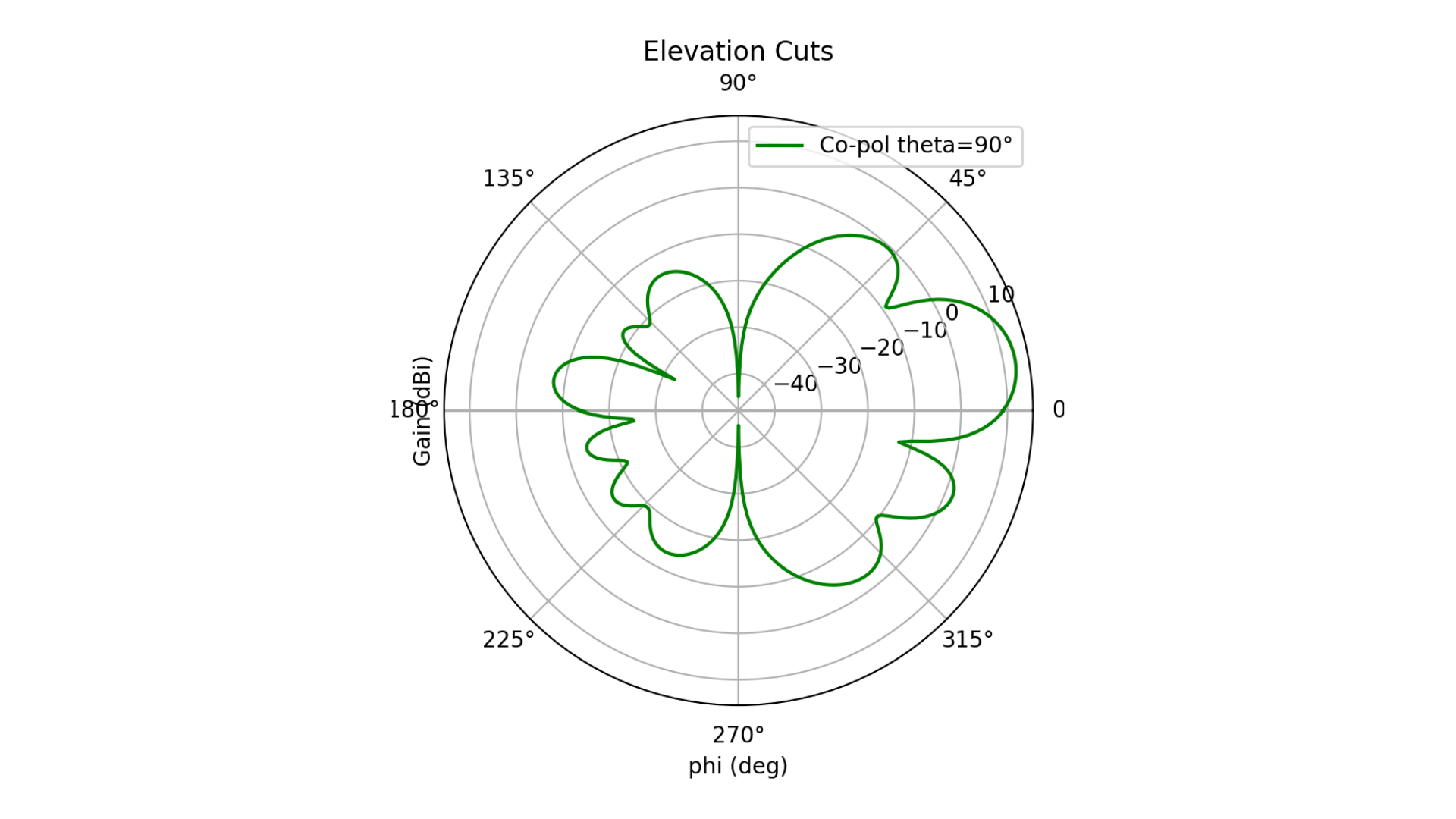
Fig. 4 Elevation cut, [1, 1, 1, 1], 10-degree tilt

# 3D radiation pattern

fig3d, ax3d = post_report.plotPolar3D(gain[:, :, 0, freq_idx, 1], -20.0, 20.0)

fig3d.show()

plt.show()

Fig. 5 3D radiation pattern, [1,1,1,1], 10-degree tilt

Note that the script also searches for first upper side lobe level and calculates side lobe suppression. 

Max gain = 12.61dBi at Theta=90.0deg, Phi=10.0deg

Beam tilt = 10.0deg

First upper sidelobe = -0.5dBi (SLS = 13.1dB)

By changing amplitudes variable, implement unequal amplitude distribution. 

# amplitude/phase tapering

N = w_co.shape[0]

amps = np.array([0.5, 1, 1, 0.5], dtype=float)[:N]

w_co *= amps[:, None]

The result radiation pattern has better Side Lobe Suppression Level, but lower gain.

Max gain = 12.25dBi at Theta=90.0deg, Phi=10.0deg

Beam tilt = 10.0deg

First upper sidelobe = -8.6dBi (SLS = 20.9dB)

Fig. 6 Gain over frequency and Elevation, [0.5,1,1,0.5], 10-degree tilt