Nullspace EM Tutorial Series: Bow-Tie Antenna Simulation

This is part 1 of a 6-part tutorial series hosted by experienced antenna engineer Katerina Galitskaya who is documenting her experience learning Nullspace as a new user. Over six tutorials she will progress from simulating a single bow-tie antenna to building full arrays and exploring beamforming techniques, sharing direct comparisons to other full-wave 3D EM simulation tools.

The full video version of this tutorial is available to watch on YouTube.

Problem Statement

This first tutorial covers the modeling, simulation, and post-processing of an over-the-ground printed bowtie antenna. As a more complex variant of a simple dipole antenna, the printed bowtie is widely used in cellular and space applications. In this example, we'll design a model with a central frequency of 1 GHz. The final 3D geometry is illustrated in Figure 1.

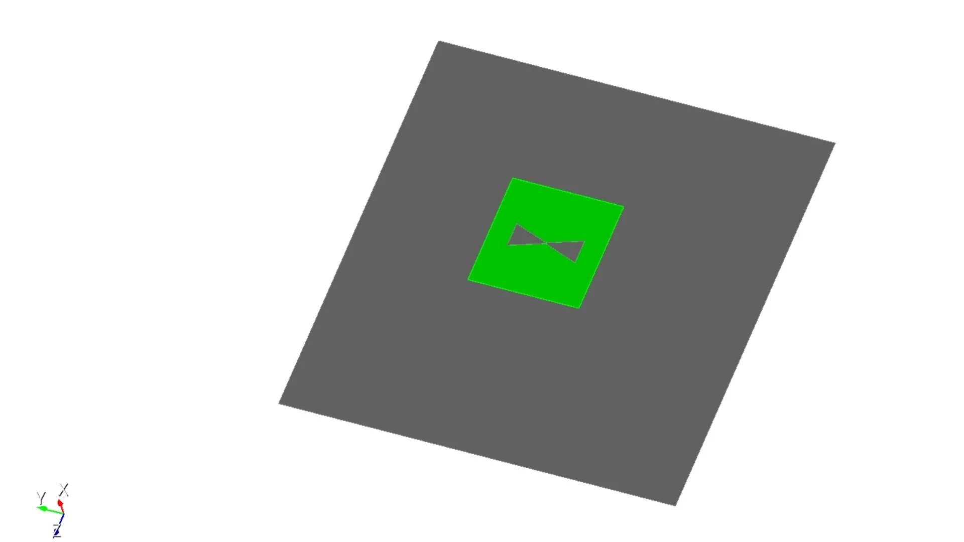
Fig. 1 Over-the-ground bow-tie antenna

Model setup

Units: CAD model is defined in millimeters, converted to meters during simulation.

Frequency sweep: 0.5–1.5 GHz (51 points).

Radiation data: Dense far‑field grid (2-degree step in theta and phi).

Extracted metrics: Return loss, input impedance, boresight gain, gain vs. frequency, 2D radiation cuts, and 3D radiation pattern.

CAD Model and Meshing

Begin by opening Prep and setting your working directory to a folder where you plan to complete this example.

Define variables for the antenna dimensions and mesh sizing. The mesh size is based on the central frequency of 1 GHz.

#{inner_width=1.7}

#{outer_width=30}

#{length_arm=42}

#{port=1.7}

#{subH=0.767}

#{subW=140}

Use the brick function to create a substrate and define two surfaces for the port. In Nullspace EM, voltage sources are implemented using the split-strip feed method. This method requires two surfaces sharing a common edge, and the source-defining curve must lie entirely within a single medium. To ensure this, we lift the two parts of the port, as shown in Figure 2.

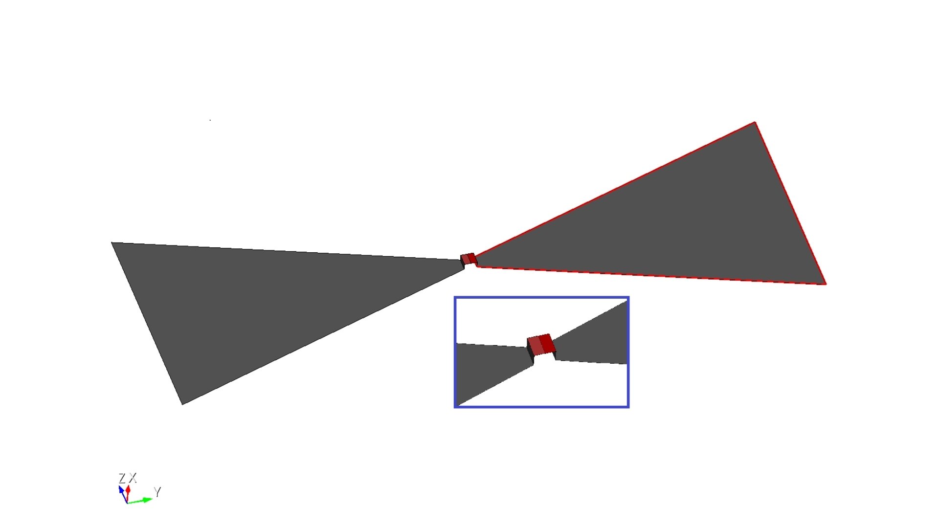
Fig. 2 Port geometry

brick x {subW} y {subW} z {subH}

volume 1 rename "substrate"

move Volume substrate z {-subH/2} include_merged ###moving the substrate to 0 on Z axis

create vertex {-port/2} {-port/2} 0 ###port structure

#{v1 = Id("vertex")}

create vertex {port/2} {-port/2} 0

create vertex {port/2} {-port/2} {port/2}

create vertex {-port/2} {-port/2} {port/2}

create surface vertex {v1} to {v1+3} 

#{port_neg_riser = Id("surface")} 

surface {port_neg_riser} copy reflect y ###reflecting one part of the port structure to create another one

#{port_pos_riser = Id("surface")}

create vertex {-port/2} {-port/2} {port/2} 

#{v1 = Id("vertex")}

create vertex {port/2} {-port/2} {port/2}

create vertex {port/2} {0} {port/2}

create vertex {-port/2} {0} {port/2}

The line {v1 = Id("vertex")} is particularly useful. It captures the ID of the most recently created vertex entity. Since Nullspace Prep renumbers entities dynamically based on operations performed, assigning IDs to variables avoids confusion and manual tracking. These IDs become APREPRO variables, enabling mathematical operations. For example, covering the vertices with a surface:

create surface vertex {v1} to {v1+3}

#{port_neg = Id("surface")}

surface {port_neg} copy reflect y 

#{port_pos = Id("surface")}

Define the shape of the bow-tie antenna using four straight-line segments. To facilitate proper meshing, perform two projection operations: firstly, project the port surfaces onto the top surface of the substrate and imprint them into the volume; secondly, project the entire bow-tie shape onto the bottom surface of the substrate.

Since the equivalent currents on the bottom of the substrate behave similarly to those on a dipole, this approach helps achieve more accurate results efficiently. 

create curve location {-outer_width/2} {port/2+length_arm} 0 location {outer_width/2} {port/2+length_arm} 0 ### the first curve of a bow-tie shape

#{c1 = Id("curve")} ### creating a variable for the curve ID

create curve location {-outer_width/2} {port/2+length_arm} 0 location {-inner_width/2} {port/2} 0 ### the second curve of a bow-tie shape

create curve location {outer_width/2} {port/2+length_arm} 0 location {inner_width/2} {port/2} 0 ### the third curve of a bow-tie shape

create curve location {-inner_width/2} {port/2} 0 location {inner_width/2} {port/2} 0 ### the fourth curve of a bow-tie shape

create surface curve {c1} to {c1+3} ### covering the 4 curves with a surface

#{dipole_top = Id("surface")} ###capturing ID of the new surface

surface {dipole_top} copy reflect y nomesh  ###reflecting the first dipole arm to create another one

#{dipole_bot = Id("surface")}

project surface {port_pos} {port_neg} onto surface 1 imprint

project surface {port_pos} {port_neg} {dipole_top} {dipole_bot} onto surface 2 imprint

The last step in creating the antenna geometry is defining the ground plane. The spacing between the antenna and the ground plane affects the radiation pattern and impedance matching. In this example, a distance of approximately a quarter wavelength is used.

create surface rectangle width 300 zplane 

#{sGND = Id("surface")}

#{vGND = Id("volume")}

#{gnd_H = 70} ### new variable for the distance between the antenna and the ground plane

move Volume {vGND} z {-gnd_H} include_merged

rotate Volume all angle 90 about Y include_merged 

imprint all

merge all

Materials & Voltage Sources

Use the provided Python script material.py to define a material library. Only FR-4 and PEC are used in this example. Open the Nullspace EM environment and load the material.py file before assigning materials.

from nsem import *

ml=MaterialLibrary()

ml.add_material(Material('FR-4', 'green', MaterialProperty('constant',real=4.4, losstan=0.02), MaterialProperty('constant',real=1.0, imag=0.0)))

ml.save('materials')

Assign the materials and define the voltage source by referencing stored surface IDs.

nsem load material library 'materials.h5'

nsem assign volume substrate material 'FR-4' ###substate material

nsem assign surface {dipole_top} {dipole_bot} material 'PEC' ###antenna arms material

nsem voltage source 'port1' pos surface {port_pos} neg surface {port_neg} impedance 50

nsem assign surface {sGND} material 'PEC' ### ground plane material

Meshing

Group the two port surfaces for easier reference and assign appropriate mesh sizes.

group 'feed' add surface {port_pos} {port_neg}

Assign the port mesh keeping in mind that the curve common to the voltage source surfaces for each feed should have a single mesh edge. 

curve common_to surface in feed interval 1

mesh surface in feed

Apply a denser mesh to the antenna arms for improved accuracy. Assign mesh to the rest of the model normally.

surface all scheme pave

#{mesh=0.3/1.5*1000/10} ###new variable for mesh size

group 'feed' add surface {port_pos} {port_neg}

curve common_to surface in feed interval 1

mesh surface in feed

surface {port_pos_riser} {port_neg_riser} interval 1

mesh surface {port_pos_riser} {port_neg_riser}

surface {dipole_top} {dipole_bot} size {mesh/4} ###meshing the antenna part

mesh surface {dipole_top} {dipole_bot} 

surface 16 18 19 20 size {mesh/4} ### meshing projections

mesh surface 16 18 19 20

surface not is_meshed in volume substrate size {mesh/4} ###meshing substrate

mesh surface not is_meshed in volume substrate

surface {sGND} size {mesh/1.5} ### meshing ground plane

mesh surface {sGND}

block 1 surface all

save cub5 "Bowtie.cub5" overwrite journal

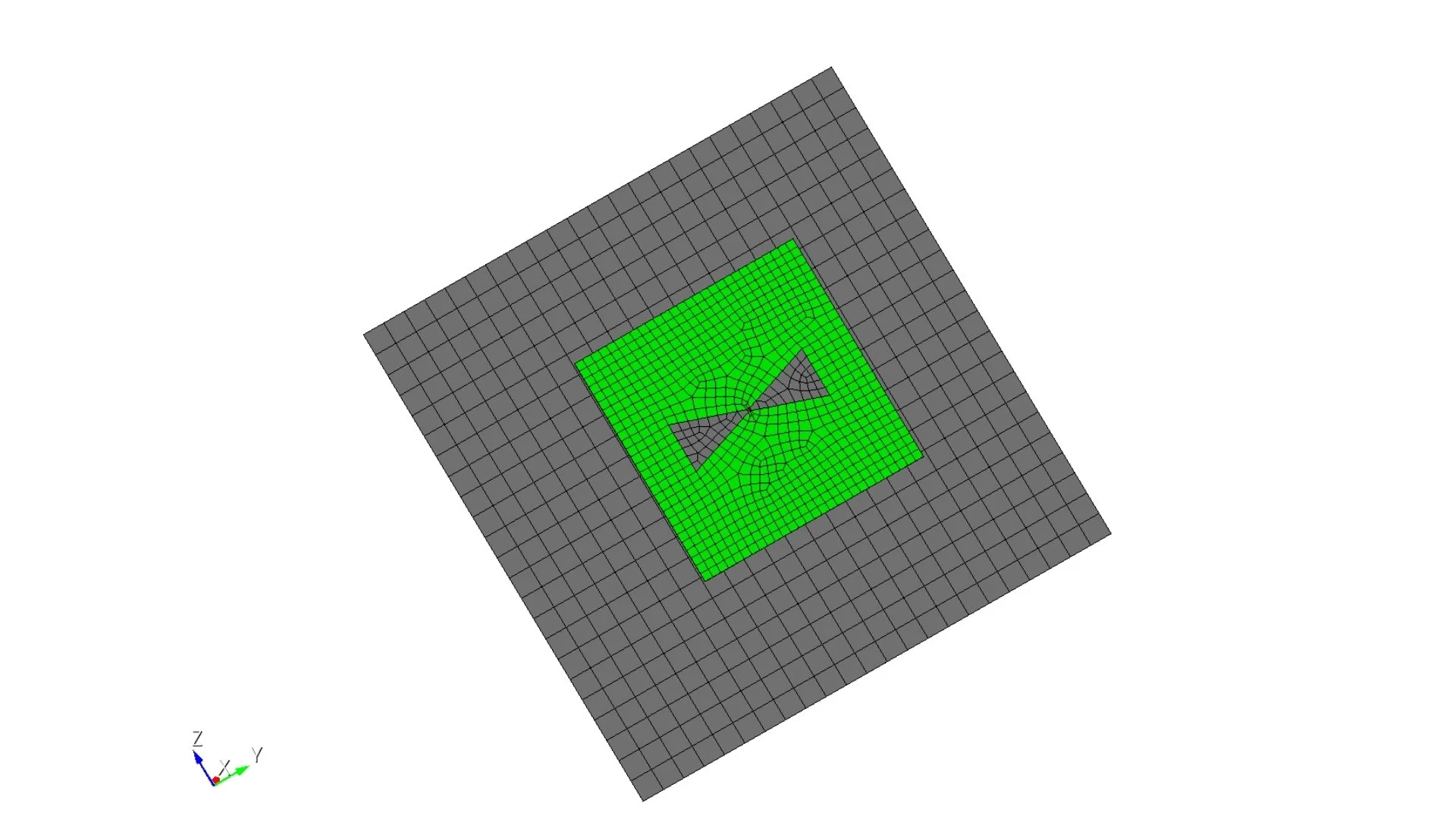
Fig.3 Model with the final mesh.

Simulation Setup

Create a simulation.py file to configure the simulation parameters.

from nsem import *

import numpy as np

config = 'Bowtie'

model = Configuration(f'{config}_sim') #configure simulation name

model.set_cub5_filename(f'{config}.cub5') #load the mesh file

model.set_order(1) #set basis order, default is 1

model.set_model_scale(0.001) #convertion to mm

model.set_frequencies(freq_beg=0.5, freq_end=1.5) #set frequency sweep from 0.5 to 1.5 GHz

model.save()

report = Report(f'{config}_report', f'{config}_sim') #create a report object

report.set_frequencies(np.linspace(0.5, 1.5, 51))

step = 2 #set the step for theta and phi angles 

theta_scan = np.linspace(0, 180, int(180/step+1)) #theta angles from 0 to 180 degrees

phi_scan = np.linspace(0, 360, int(360/step)) #phi angles from 0 to 360 degrees

report.request_far_fields_grid(theta_scan, phi_scan) #request far-field data

report.save() #save the report configuration

model.run() #run the simulation

report.run() #run the report generation

Post-Processing

Create postprocessing.py to extract simulation data and visualize results.

import matplotlib.pyplot as plt

import numpy as np

from nsem.postprocessing import *  

config = 'Bowtie_v2025'

post = PostProcess(f'{config}_sim')  #create a post-processing object for the simulation

freq = post.get_frequencies()  #get frequencies from the simulation

freq = np.linspace(np.min(freq), np.max(freq), 51)  #create a frequency array for evaluation

sparam = post.get_s_parameters(freq_evaluate=freq)  #get S-parameters

rl = dB20(np.squeeze(sparam[0, 0, :]))  # convert S-parameters to dB scale

impedance = post.get_input_impedance(freq_evaluate=freq)  #get input impedance

impedance_real = np.real(np.squeeze(impedance[0, :]))  #get the real part of the input impedance

impedance_imag = np.imag(np.squeeze(impedance[0, :]))  #get the imaginary part of the input impedance

#plots

fig = plt.figure(figsize=(18, 12))

ax1 = plt.subplot2grid((2,3),(0,0))

ax2 = plt.subplot2grid((2,3),(0,1))

ax3 = plt.subplot2grid((2,3),(0,2))

ax4 = plt.subplot2grid((2,3),(1,0), polar = True)

ax5 = plt.subplot2grid((2,3),(1,1), polar = True)

ax6 = plt.subplot2grid((2,3),(1,2))

#return loss

ax1.plot(freq, rl, label='S11', color='blue')

ax1.set_xlabel('Frequency (GHz)')

ax1.set_ylabel('dB')

ax1.set_title('S-parameters')

ax1.grid(True)

ax1.legend()    

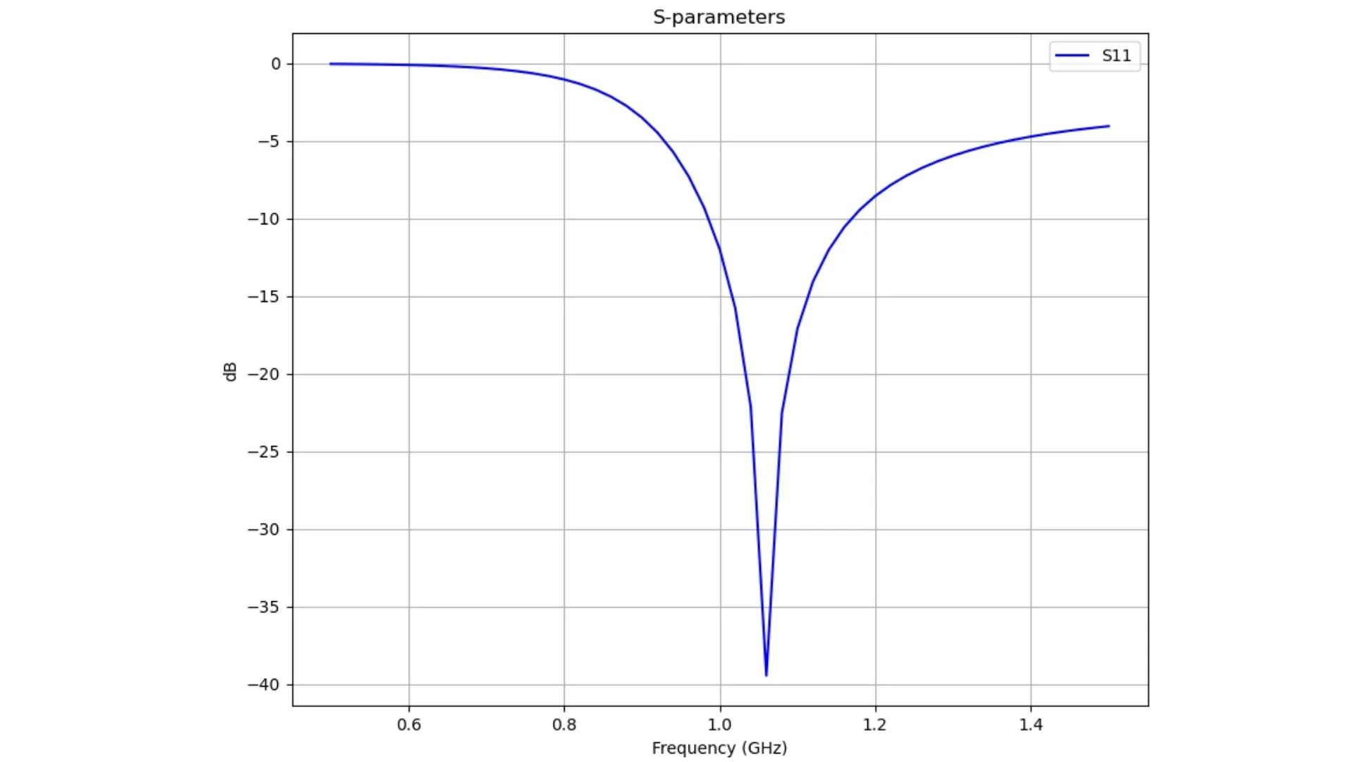
Fig. 4 Return loss plot

#impedance

ax2.plot(freq, impedance_real, label='Re(Z)', color='red')

ax2.plot(freq, impedance_imag, label='Im(Z)', color='orange')

ax2.set_xlabel('Frequency (GHz)')

ax2.set_ylabel('impedance')

ax2.grid(True)

ax2.legend()

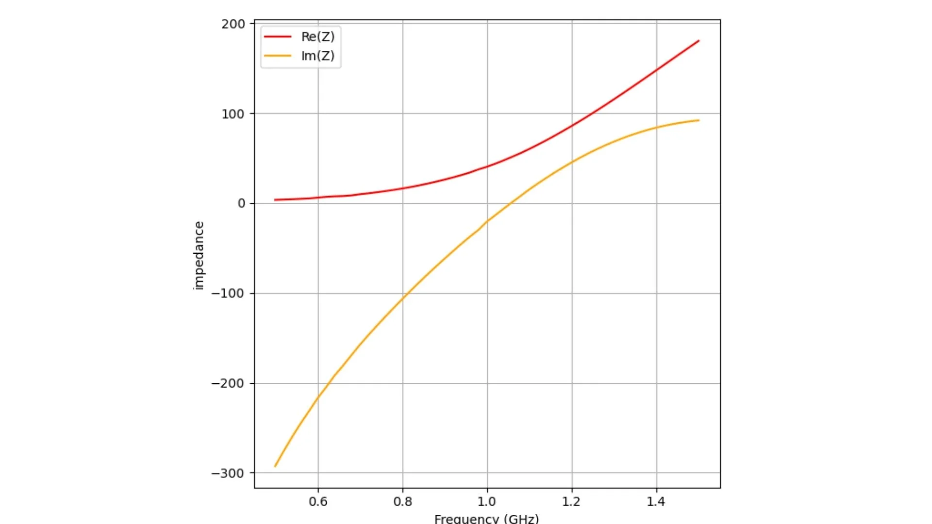
Fig. 5 Impedance plot

post = PostProcess(f'{config}_report') # create a post-processing object for the report

gain = post.get_gain('spherical')

theta = post.get_obs_theta()

phi = post.get_obs_phi()

theta_idx, theta_val = post.get_nearest(theta, 0.0)

phi0_idx, _ = post.get_nearest(phi, 0.0)

phi90_idx, _ = post.get_nearest(phi, 90.0)

theta90_idx, _ = post.get_nearest(theta, 90.0)

freq_idx, freq_val = post.get_nearest(freq, 1)

gain_0= np.squeeze(gain[phi0_idx, theta90_idx, 0, :, 1])  # get the max gain

gain_copol_theta90 = gain[:, theta90_idx, 0, freq_idx, 1]   

gain_xpol_theta90 = gain[:, theta90_idx, 0, freq_idx, 0]

#Gain

ax3.plot(freq, gain_0, label='Gain max', color='blue')

ax3.set_xlabel('Frequency')

ax3.set_ylabel('Gain (dB)')

ax3.set_title('Gain')

ax3.grid(True)

ax3.legend()

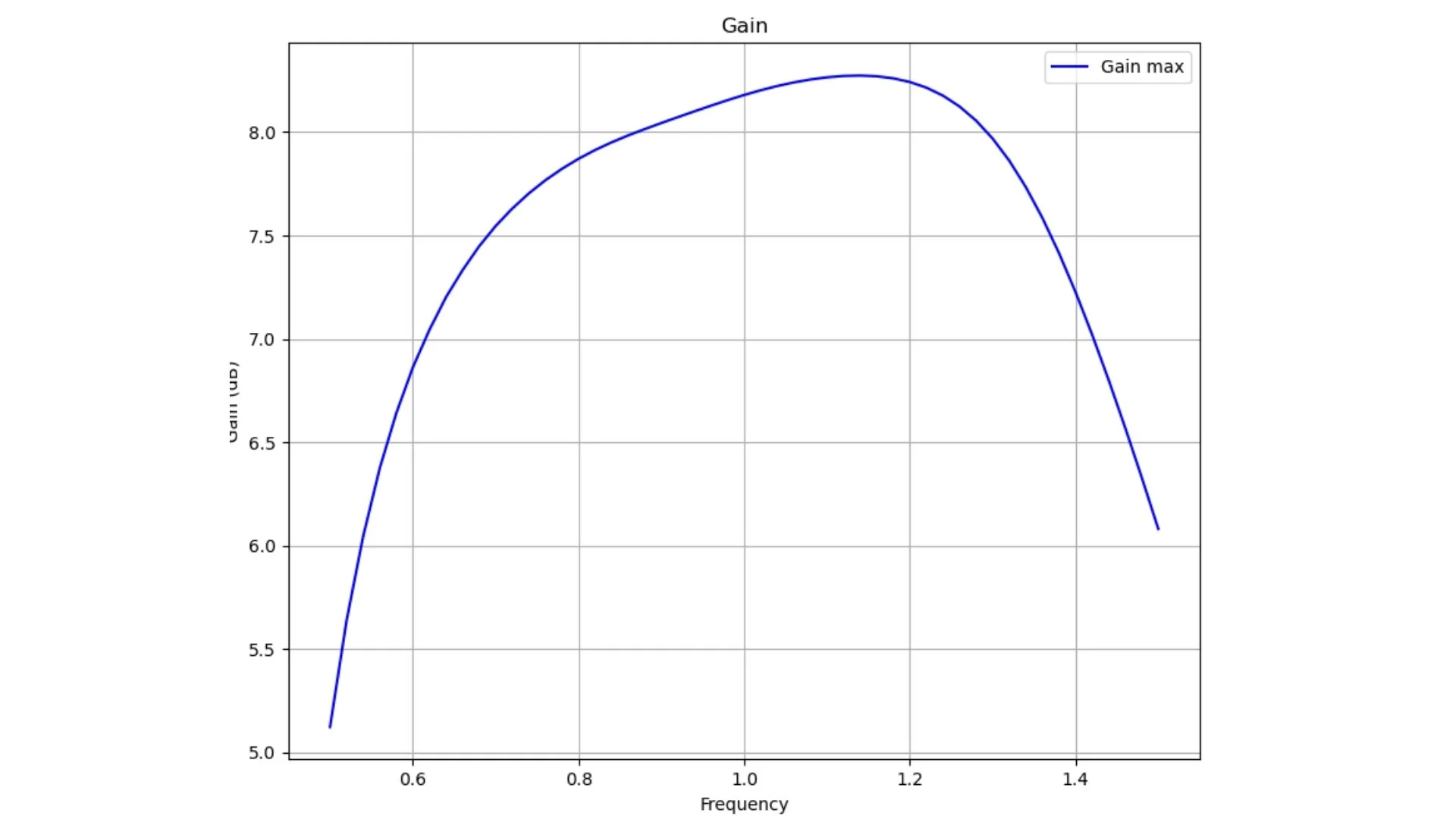
Fig. 6 Boresight gain over frequency

#pattern cut

ax4.plot(np.deg2rad(phi), gain_copol_theta90, label='Theta 90 copol', color='blue')

ax4.set_xlabel('Phi (deg)')

ax4.set_ylabel('Gain (dB)')

ax4.set_ylim([-30, 10])

ax4.grid(True)

ax4.legend()

fig.tight_layout()

fig.delaxes(ax6)  

fig.delaxes(ax5)  

Fig. 7 Gain plot along phi, theta = 90

#3D radiation pattern

fig3d,ax3d = post.plotPolar3D(gain[:,:,0,freq_idx,1], -10.0,10.0)

fig3d.show()

plt.show()

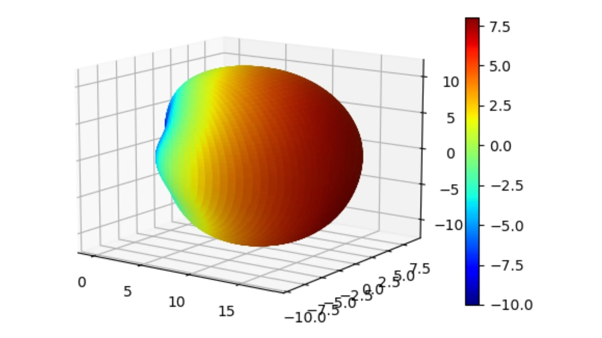
Fig. 8 3D gain pattern