This is part 4 of a 6-part tutorial series hosted by experienced antenna engineer Katerina Galitskaya who is documenting her experience learning Nullspace as a new user. Over six tutorials she will progress from simulating a single bow-tie antenna to building full arrays and exploring beamforming techniques, sharing direct comparisons to other full-wave 3D EM simulation tools.
Problem Statement
This tutorial presents the modeling, simulation, and post-processing of a 4-element antenna array enclosed in a glass fiber radome. The radome effect is a crucial factor when working with antenna arrays, as it can detune the elements and reduce realized gain. The final 3D geometry is shown in Figure 1.
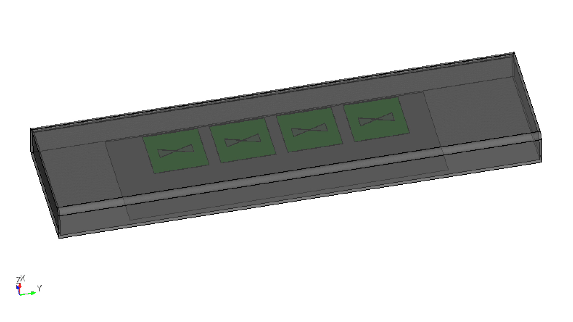
Fig. 1 Antenna array with a radome
Model setup
Preparation: Use the antenna array model from the third tutorial.
Units: CAD model is defined in millimeters, converted to meters during simulation.
Frequency sweep: 0.5–1.5 GHz (51 points).
Radiation data: Dense far‑field grid (2-degree step in theta and phi).
Extracted metrics: Active S-parameters, boresight gain, gain vs. frequency, 2D radiation cuts, and 3D radiation pattern.
CAD Model and Meshing
Begin by opening Prep and setting your working directory to a folder where you plan to complete this example.
Complete the modeling of a 4-element antenna array as described in the previous tutorial.
#{inner_width=1.7}#{outer_width=30}
#{leng=42}
#{port=1.7}
#{subH=0.767}
#{subW=140}
###substrate geometry
brick x {subW} y {subW} z {subH}
volume 1 rename "substrate"
move Volume substrate z {-subH/2} include_merged
###ports geometry
create vertex {-port/2} {-port/2} 0
#{v1 = Id("vertex")}
create vertex {port/2} {-port/2} 0
create vertex {port/2} {0} {port/4}
create vertex {-port/2} {0} {port/4}
create surface vertex {v1} to {v1+3}
#{port_pos = Id("surface")}
surface {port_pos} copy reflect y
#{port_neg = Id("surface")}
###antenna geometry
create curve location {-outer_width/2} {port/2+leng} 0 location {outer_width/2} {port/2+leng} 0
#{c1 = Id("curve")}
create curve location {-outer_width/2} {port/2+leng} 0 location {-inner_width/2} {port/2} 0
create curve location {outer_width/2} {port/2+leng} 0 location {inner_width/2} {port/2} 0
create curve location {-inner_width/2} {port/2} 0 location {inner_width/2} {port/2} 0
create surface curve {c1} to {c1+3}
#{dipole_top = Id("surface")}
surface {dipole_top} copy reflect y nomesh
#{dipole_bot = Id("surface")}
project surface {port_pos} {port_neg} onto surface 1 imprint
project surface {port_pos} {port_neg} {dipole_top} {dipole_bot} onto surface 2 imprint
###ground plane
create surface rectangle width 300 zplane
#{GND = Id("surface")}
#{gnd_H=70}
move Volume 6 z {-gnd_H} include_merged preview
move Volume 6 z {-gnd_H} include_merged
###4-element array creation
Volume 1 2 3 4 5 6 copy move x 0 y 170 z 0 repeat 3 group_results
unite surface {GND} 36 53 70
#{GND = Id("surface")}
Import the STEP file for the radome. Ensure that the file path is correctly specified.
import step "INSERT PATH HERE/radome.step" heal group "radome" ### importing step file of the radome
#{radome = Id("volume")} ### getting a variable for the radome volume ID
move volume {radome} y -170 include_merged #### center the radome to array geometry
rotate Volume all angle 90 about Y include_merged preview
rotate Volume all angle 90 about Y include_merged
imprint all
merge all
Materials & Voltage Sources
Use the material.py script to define the material library. In this example, we add glass fiber to the existing materials (FR-4 and PEC). Open the Nullspace EM environment and load the material.py file before assigning materials.
from nsem import *
ml=MaterialLibrary()
ml.add_material(Material('FR-4', 'green', MaterialProperty('constant',real=4.4, losstan=0.02), MaterialProperty('constant',real=1.0, imag=0.0)))
ml.add_material(Material('glassfiber', 'grey', MaterialProperty('constant',real=4.7, losstan=0.09), MaterialProperty('constant',real=1.0, imag=0.0)))
ml.save('materials')
Assign materials and define four voltage sources. Ensure consistent assignment of positive and negative terminals across all ports.
nsem load material library 'materials.h5'
nsem assign volume substrate material 'FR-4' ###the original substrate
nsem assign volume 7 13 19 material 'FR-4' ###the 3 copies
nsem assign volume {radome} material 'glassfiber' ### glass fiber material to the radome
nsem assign surface {dipole_top} {dipole_bot} material 'PEC' ###the original antenna
nsem assign surface 34 35 36 51 52 53 68 69 70 material 'PEC' ###the 3 copies
nsem voltage source 'port_001' pos surface {port_pos} neg surface {port_neg} impedance 50
nsem voltage source 'port_002' pos surface 32 neg surface 33 impedance 50
nsem voltage source 'port_003' pos surface 49 neg surface 50 impedance 50
nsem voltage source 'port_004' pos surface 66 neg surface 67 impedance 50
nsem assign surface {GND} material 'PEC'
Meshing
Repeat the meshing as shown in the previous tutorial. Use lambda/10 meshing for the radome part.
###meshing
surface all scheme pave
#{mesh=0.3/1*1000/10}
group 'feed' add surface {port_pos} {port_neg} 32 33 49 50 66 67
curve common_to surface in feed interval 1
mesh surface in feed
surface {dipole_top} {dipole_bot} 34 35 51 52 68 69 size {mesh/4}
mesh surface {dipole_top} {dipole_bot} 34 35 51 52 68 69
surface 14 16 17 18 size {mesh/4}
mesh surface 14 16 17 18
surface {GND} size {mesh/1.5}
mesh surface {GND}
surface not is_meshed in volume 1 7 13 19 size {mesh/4}
mesh surface not is_meshed in volume 1 7 13 19
surface not is_meshed in volume {radome} size {mesh}
mesh surface not is_meshed in volume {radome}
block 1 surface all
#save cub5 "radome_array.cub5" overwrite journal
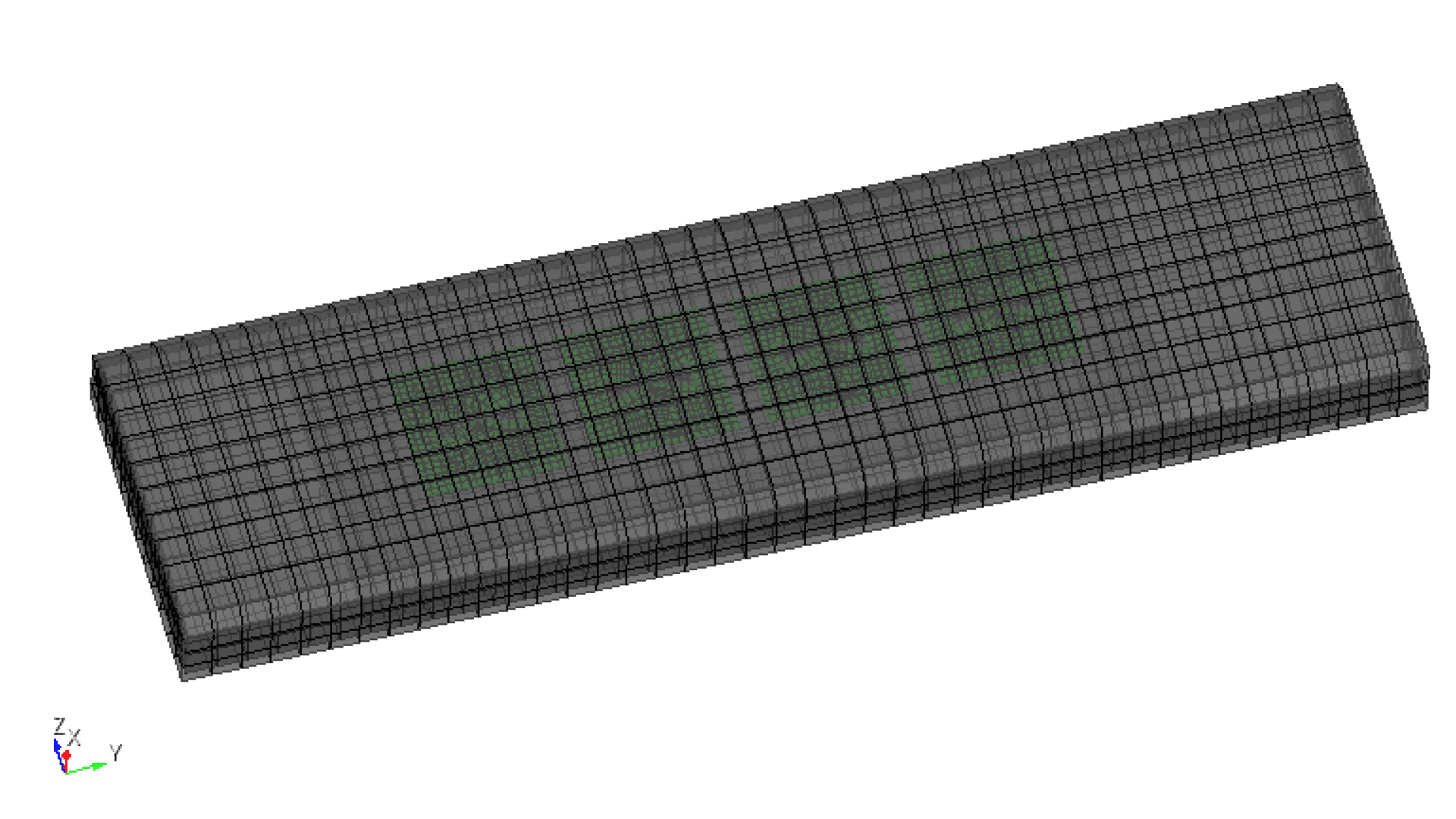
Fig.2 Model with the final mesh.
Simulation Setup
Create a simulation.py file to configure the simulation parameters.
from nsem import *
import numpy as np
config = 'radome_array'
model = Configuration(f'{config}_sim') #configure simulation name
model.set_cub5_filename(f'{config}.cub5') #load the mesh file
model.set_order(1) #set basis order, default is 1
model.set_model_scale(0.001) #convertion to mm
model.set_frequencies(freq_beg=0.5, freq_end=1.5) #set frequency sweep from 0.5 to 1.5 GHz
model.save()
report = Report(f'{config}_report', f'{config}_sim') #create a report object
report.set_frequencies(np.linspace(0.5, 1.5, 11))
step = 2 #set the step for theta and phi angles
theta_scan = np.linspace(0, 180, int(180/step+1)) #theta angles from 0 to 180 degrees
phi_scan = np.linspace(0, 360, int(360/step)) #phi angles from 0 to 360 degrees
report.request_far_fields_grid(theta_scan, phi_scan) #request far-field data
report.save() #save the report configuration
model.run() #run the simulation
report.run() #run the report generation
Post-Processing
Create postprocessing.py to extract simulation data and visualize results.
import matplotlib.pyplot as plt
import numpy as np
from nsem.postprocessing import *
from scipy.interpolate import CubicSpline
config = 'radome_array'
post = PostProcess(f'{config}_sim') # create a post-processing object for the simulation
freq = post.get_frequencies() # get the frequencies
freq = np.linspace(np.min(freq), np.max(freq), 501) # create a frequency array for evaluation
w = [1.0, 1.0, 1.0, 1.0] # excitation of each port
active_s = post.get_active_s_parameters(freq_evaluate=freq,weights=w)
active_s11 = dB20(np.squeeze(active_s[0, :]))
active_s22 = dB20(np.squeeze(active_s[1, :]))
active_s33 = dB20(np.squeeze(active_s[2, :]))
active_s44 = dB20(np.squeeze(active_s[3, :]))
#plots
fig = plt.figure(figsize=(18, 6))
ax1 = plt.subplot(1, 3, 1)
ax2 = plt.subplot(1, 3, 2)
ax3 = plt.subplot(1, 3, 3, polar=True)
# active S-parameters
ax1.plot(freq, active_s11, label='active S11', color='blue')
ax1.plot(freq, active_s22, label='active S22', color='orange')
ax1.plot(freq, active_s33, label='active S33', color='green')
ax1.plot(freq, active_s44, label='active S44', color='red')
ax1.set_xlabel('Frequency (GHz)')
ax1.set_ylabel('S11 (dB)')
ax1.set_title('Active S-parameters')
ax1.grid(True)
ax1.legend()
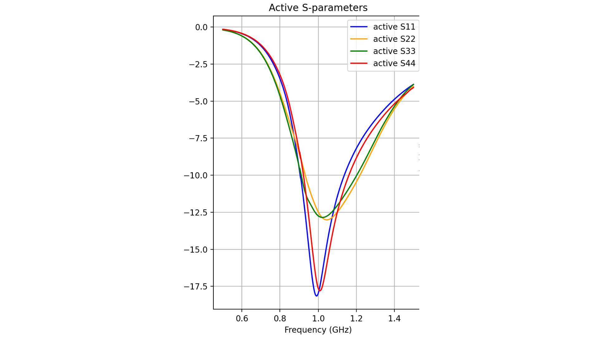
Fig. 3 Active S11 for each port
post = PostProcess(f'{config}_report') # create a post-processing object for the report
freq = post.get_frequencies()
theta = post.get_obs_theta()
phi = post.get_obs_phi()
gain = post.get_gain('spherical',weights=w) #get gain with specified amplitude/phase distribution
theta_idx,_ = post.get_nearest(theta, 0.0)
phi0_idx,_ = post.get_nearest(phi, 0.0)
phi90_idx,_ = post.get_nearest(phi, 90.0)
theta90_idx,_ = post.get_nearest(theta, 90.0)
theta0_idx,_ = post.get_nearest(theta, 0.0)
freq_idx,_ = post.get_nearest(freq, 1.0)
gain_0 = gain[phi0_idx, theta90_idx, 0, freq_idx, 1]
print(f"Boresight gain (dBi): {gain_0:.2f}")
gain_copol_phi0 = gain[phi0_idx, :, 0, freq_idx,1]
gain_copol_phi90 = gain[phi90_idx, :, 0, freq_idx, 0]
gain_xpol_phi0 = gain[phi0_idx, :, 0, freq_idx, 0]
gain_xpol_phi90 = gain[phi90_idx, :, 0, freq_idx, 1]
gain_copol_theta90 = gain[:, theta90_idx, 0, freq_idx, 1]
gain_xpol_theta90 = gain[:, theta90_idx, 0, freq_idx, 0]
#Gain plot interpolation
gain_max = np.squeeze(gain[phi0_idx, theta90_idx, 0, :, 1])
x = np.asarray(freq).ravel()
y = np.asarray(gain_max).ravel()
x_unique, idx = np.unique(x, return_index=True)
y_unique = y[idx]
cs = CubicSpline(x_unique, y_unique, bc_type='natural', extrapolate=False)
x_dense = np.linspace(x_unique[0], x_unique[-1], 501)
y_dense = cs(x_dense)
# Gain vs frequency
ax2.plot(x_dense, y_dense, label='Gain with radome', color='blue')
ax2.set_xlabel('Frequency (GHz)')
ax2.set_ylabel('Gain (dBi)')
ax2.set_title('Boresight Gain vs Frequency')
ax2.grid(True)
ax2.legend()
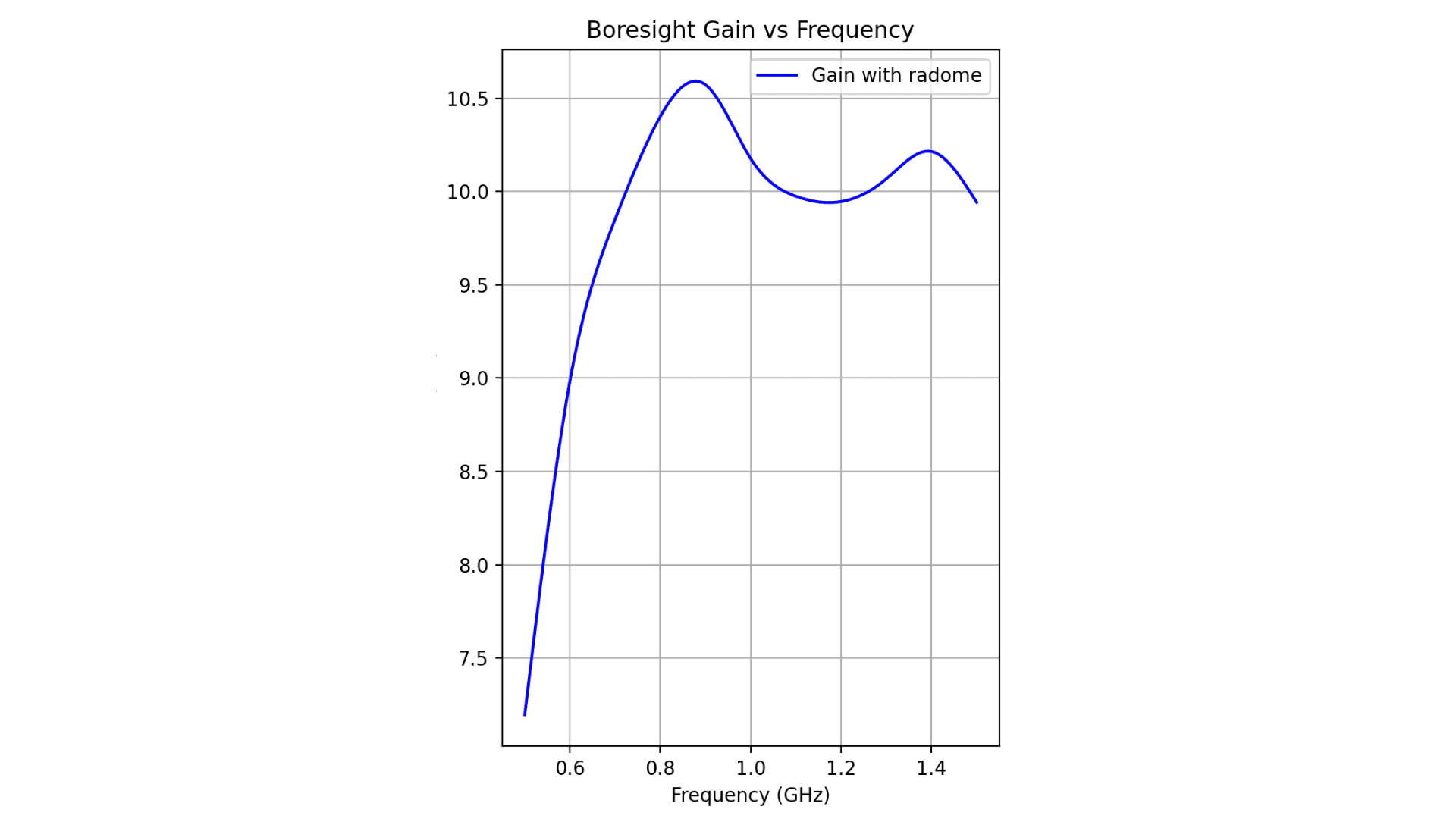
Fig. 4 Boresight gain over frequency
# Elevation cut
ax3.plot(np.deg2rad(phi), gain_copol_theta90, label=f'Co-pol theta=90°', color='green')
ax3.set_xlabel('phi (deg)')
ax3.set_ylabel('Gain (dBi)')
ax3.set_title('Elevation Cuts')
ax3.grid(True)
ax3.legend()
fig.tight_layout()
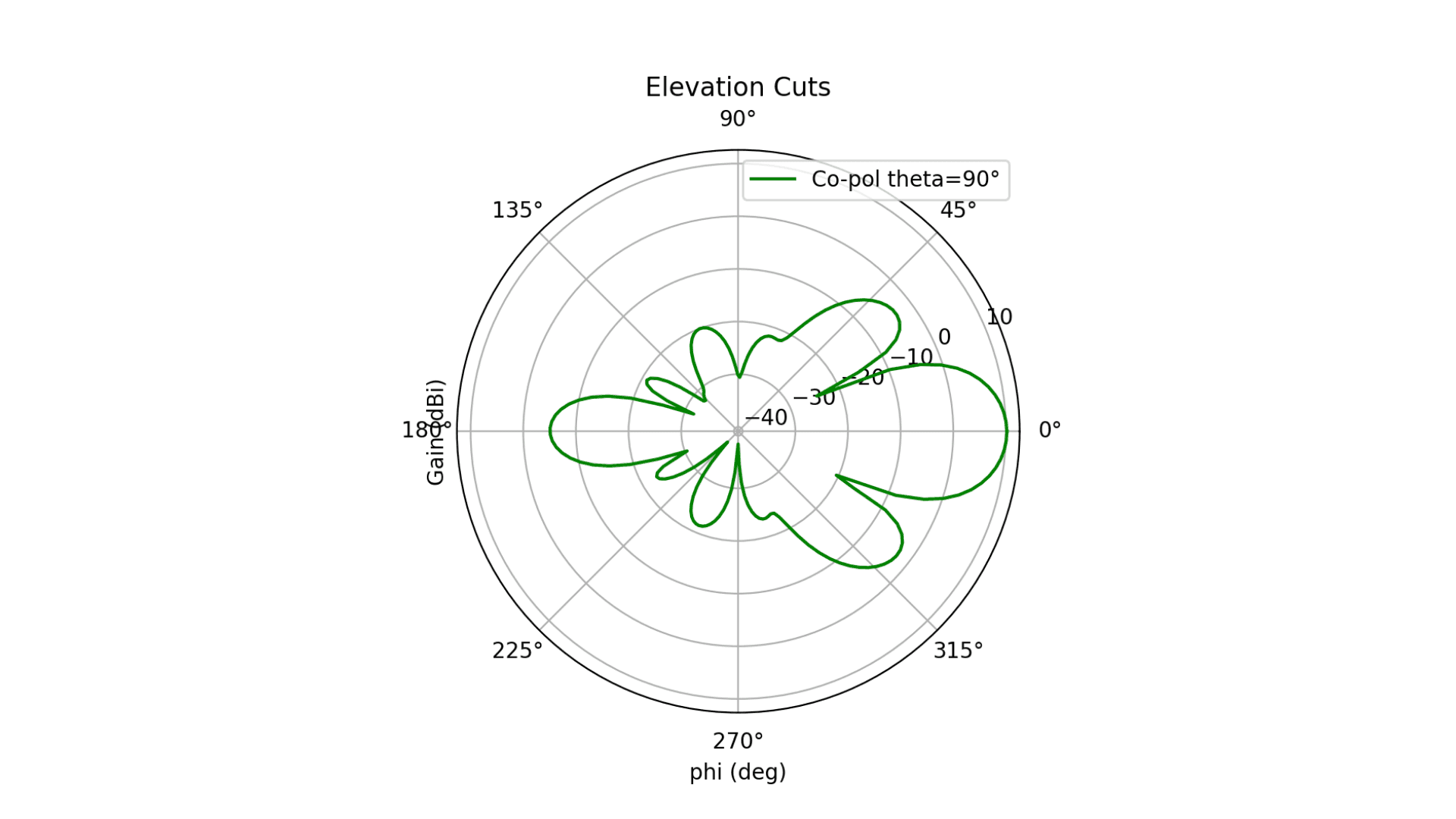
Fig. 5 Gain plot along phi, theta = 90
#3D radiation pattern
fig3d,ax3d = post.plotPolar3D(gain[:,:,0,freq_idx,1], -20.0,20.0)
fig3d.show()
plt.show()
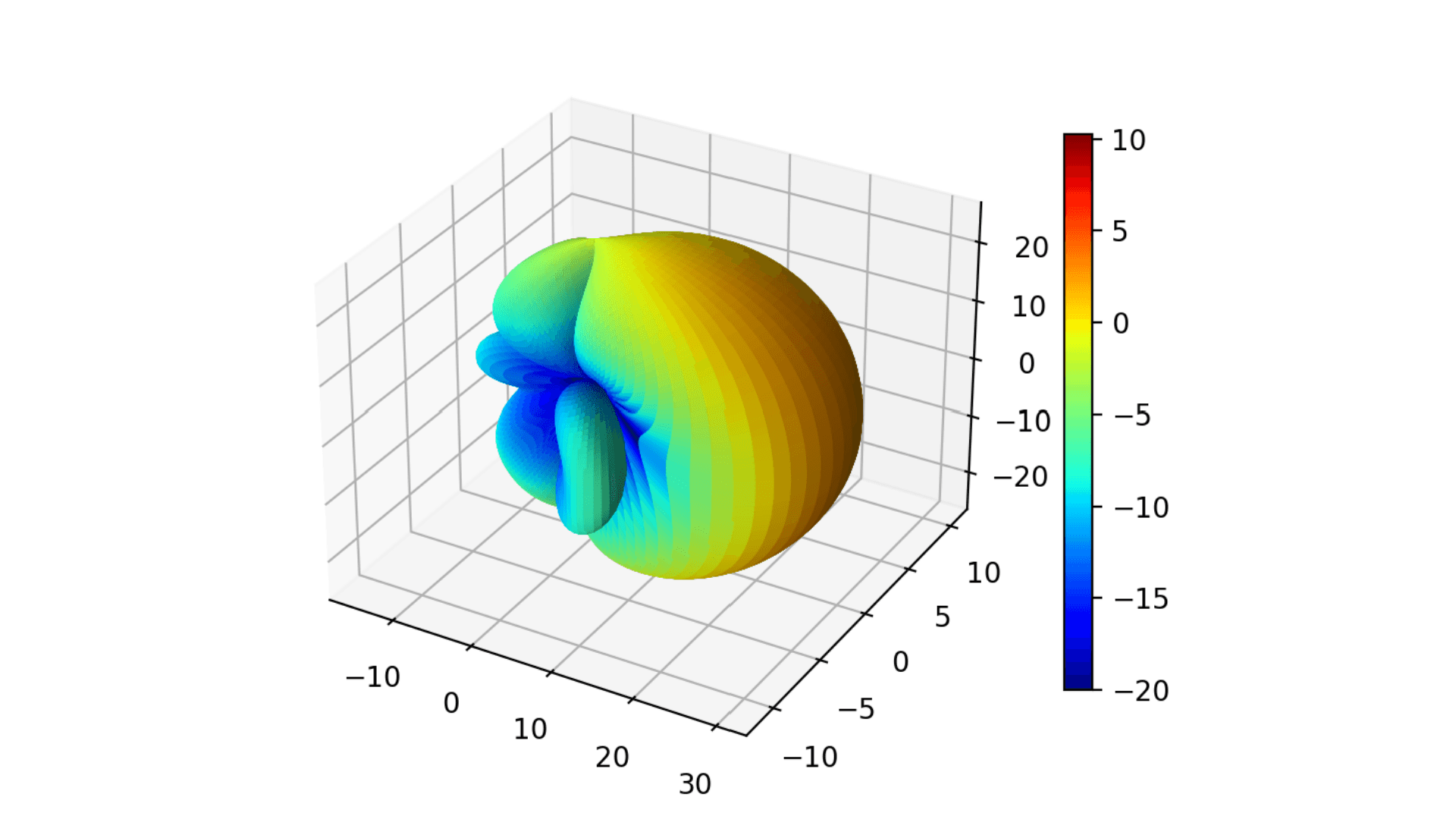
Fig. 6 3D gain pattern