This is the last of our 6-part tutorial series hosted by experienced antenna engineer Katerina Galitskaya who is documenting her experience learning Nullspace as a new user. Over six tutorials she progresses from simulating a single bow-tie antenna to building full arrays and exploring beamforming techniques, sharing direct comparisons to other full-wave 3D EM simulation tools.
Problem Statement
This tutorial covers the modeling, simulation, and post-processing of an electrically large problem consisting of two 4-element antenna arrays mounted on a 10-meter telecom tower. Modern cellular sites commonly host multiple antennas, making mutual coupling a critical performance consideration. The completed 3D geometry is shown in Figure 1.
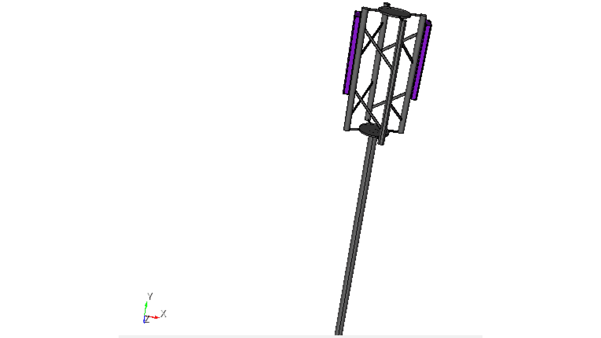
Fig. 1 Two integrated antenna arrays on a tower
Model setup
Preparation: Use the installed antenna array model from the fifth tutorial.
Units: CAD model is defined in millimeters, converted to meters during simulation.
Frequency sweep: 0.5–1.5 GHz (11 points).
Radiation data: Dense far‑field grid (2-degree step in theta and phi).
Extracted metrics: S21 coupling between antennas, boresight gain, gain vs. frequency, 2D radiation cuts, and 3D radiation pattern.
CAD Model and Meshing
Begin by opening Prep and setting your working directory to a folder where you plan to complete this example.
Use the parameter definitions and modeling instructions from the previous tutorial.
#{inner_width=1.7}
#{outer_width=30}
#{leng=42}
#{port=1.7}
#{subH=0.767}
#{subW=140}
###substrate geometry
brick x {subW} y {subW} z {subH}
volume 1 rename "substrate"
move Volume substrate z {-subH/2} include_merged
###ports geometry
create vertex {-port/2} {-port/2} 0
#{v1 = Id("vertex")}
create vertex {port/2} {-port/2} 0
create vertex {port/2} {0} {port/4}
create vertex {-port/2} {0} {port/4}
create surface vertex {v1} to {v1+3}
#{port_pos = Id("surface")}
surface {port_pos} copy reflect y
#{port_neg = Id("surface")}
###antenna geometry
create curve location {-outer_width/2} {port/2+leng} 0 location {outer_width/2} {port/2+leng} 0
#{c1 = Id("curve")}
create curve location {-outer_width/2} {port/2+leng} 0 location {-inner_width/2} {port/2} 0
create curve location {outer_width/2} {port/2+leng} 0 location {inner_width/2} {port/2} 0
create curve location {-inner_width/2} {port/2} 0 location {inner_width/2} {port/2} 0
create surface curve {c1} to {c1+3}
#{dipole_top = Id("surface")}
surface {dipole_top} copy reflect y nomesh
#{dipole_bot = Id("surface")}
project surface {port_pos} {port_neg} onto surface 1 imprint
project surface {port_pos} {port_neg} {dipole_top} {dipole_bot} onto surface 2 imprint
###ground plane
create surface rectangle width 300 zplane
#{GND = Id("surface")}
#{gnd_H=70}
move Volume 6 z {-gnd_H} include_merged
###4-element array creation
Volume 1 2 3 4 5 6 copy move x 0 y 170 z 0 repeat 3 group_results
unite surface {GND} 36 53 70
#{GND = Id("surface")}
####radome import
import step "radome.step" heal group "radome"
#{radome = Id("volume")}
move volume {radome} y -170 include_merged
rotate Volume all angle 90 about Y include_merged preview
rotate Volume all angle 90 about Y include_merged
###tower import
import step "TelecomMast_simplified.step" heal group "Tower"
#{tower = Id("volume")}
move volume {tower} x -580 y -11000 z 130 include_merged
### Remove small features and surfaces from tower model
remove surface 181, 200 connected_sets
remove surface 88, 170, 199 connected_sets
select surface 183 include similar
remove surface 179, 183 connected_sets
select surface 198 118 203 include similar
remove surface 118, 198, 203, 204 connected_sets
remove surface 168
remove surface 182, 201 connected_sets
remove surface 154, 202 connected_sets
remove surface 180
remove surface 184
select surface 143 207 include similar
remove surface 143, 151, 206, 207 connected_sets
remove surface 187
remove surface 91, 92, 126 connected_sets
remove surface 122, 150, 158 connected_sets
remove surface 99, 134, 167 connected_sets
webcut volume 26 with sheet extended from surface 146
webcut volume 27 with sheet extended from surface 205
delete volume 27
remove surface 123, 127, 128 connected_sets
Copy and position the first array to the opposite pole.
Volume 1 2 3 4 5 6 7 8 9 10 11 13 14 15 16 17 19 20 21 22 23 25 copy
group 'second_array' add Volume 29 35 40 45 50 30 31 32 33 34 35 36 37 38 39 41 42 43 44 46 47 48 49
group second_array rotate 180 about Y include_merged
second_array move x -1160 y 0 z 250
imprint all
merge all
Materials & Voltage Sources
Use the material.py script to define the material library. Besides PEC, this model uses FR-4 and glass fiber. Open the Nullspace EM environment and load the material.py file before assigning materials.
from nsem import *
ml=MaterialLibrary()
ml.add_material(Material('FR-4', 'green', MaterialProperty('constant',real=4.4, losstan=0.02), MaterialProperty('constant',real=1.0, imag=0.0)))
ml.add_material(Material('glassfiber', 'grey', MaterialProperty('constant',real=4.7, losstan=0.09), MaterialProperty('constant',real=1.0, imag=0.0)))
ml.save('materials')
Assign materials and define four voltage sources per array. Ensure consistent assignment of positive and negative terminals across all ports.
###first array materials and ports
nsem load material library 'materials.h5'
nsem assign volume substrate material 'FR-4'
nsem assign volume 7 13 19 material 'FR-4'
nsem assign volume {radome} material 'glassfiber'
nsem assign surface {dipole_top} {dipole_bot} material 'PEC'
nsem assign surface 34 35 51 52 68 69 material 'PEC'
nsem assign volume {tower} 28 material 'PEC'
nsem assign surface {GND} material 'PEC'
nsem voltage source 'port_101' pos surface {port_pos} neg surface {port_neg} impedance 50
nsem voltage source 'port_102' pos surface 32 neg surface 33 impedance 50
nsem voltage source 'port_103' pos surface 49 neg surface 50 impedance 50
nsem voltage source 'port_104' pos surface 66 neg surface 67 impedance 50
###second array materials and ports
nsem assign volume 29 35 40 45 material 'FR-4'
nsem assign volume 50 material 'glassfiber'
nsem assign surface 227 226 243 244 259 260 275 276 material 'PEC'
nsem assign surface 228 material 'PEC'
nsem voltage source 'port_201' pos surface 224 neg surface 225 impedance 50
nsem voltage source 'port_202' pos surface 241 neg surface 242 impedance 50
nsem voltage source 'port_203' pos surface 257 neg surface 258 impedance 50
nsem voltage source 'port_204' pos surface 273 neg surface 274 impedance 50
Meshing
Repeat the meshing on the second array like the first one.
###meshing
surface all scheme pave
#{mesh=0.3/1*1000/10}
###first array meshing
#port meshing
group 'feed1' add surface {port_pos} {port_neg} 32 33 49 50 66 67
curve common_to surface in feed1 interval 1
mesh surface in feed1
#antenna meshing
surface {dipole_top} {dipole_bot} 34 35 51 52 68 69 size {mesh/4}
mesh surface {dipole_top} {dipole_bot} 34 35 51 52 68 69
surface 14 16 17 18 size {mesh/4}
mesh surface 14 16 17 18
surface {GND} size {mesh/1.5}
mesh surface {GND}
surface not is_meshed in volume 1 7 13 19 size {mesh/4}
mesh surface not is_meshed in volume 1 7 13 19
#radome meshing
surface not is_meshed in volume {radome} size {mesh}
mesh surface not is_meshed in volume {radome}
###second array meshing
group 'feed2' add surface 224 225 241 242 257 258 273 274
curve common_to surface in feed2 interval 1
mesh surface in feed2
#antenna meshing
surface 227 226 243 244 259 260 275 276 size {mesh/4}
mesh surface 227 226 243 244 259 260 275 276
surface 228 size {mesh/1.5}
mesh surface 228
surface not is_meshed in volume 29 35 40 45 size {mesh/4}
mesh surface not is_meshed in volume 29 35 40 45
#radome meshing
surface not is_meshed in volume 50 size {mesh}
mesh surface not is_meshed in volume 50
### telecom tower meshing
surface not is_meshed in volume {tower} size {mesh}
mesh surface not is_meshed in volume {tower}
surface not is_meshed in volume 28 size {mesh}
mesh surface not is_meshed in volume 28
block 1 surface all
quality surface all shape global draw mesh
save cub5 "two_arrays.cub5" overwrite journal
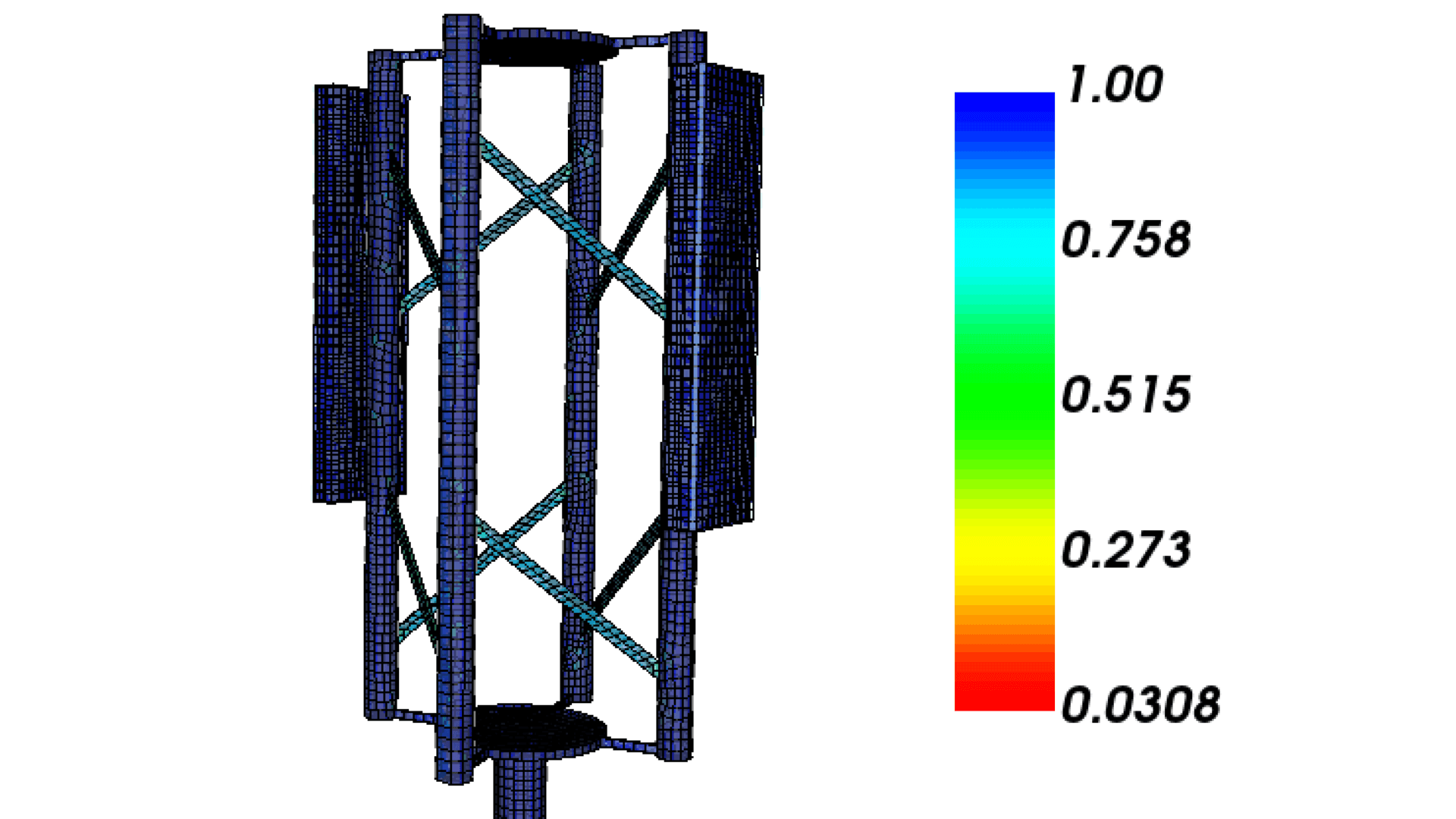
Fig. 2 Model with the mesh quality plotted.
Simulation Setup
Create a simulation.py file to configure the simulation parameters. Since the structure is electrically large, use the compression solver, which performs matrix compression and leverages near- and far-field coupling to efficiently represent the system.
from nsem import *
import numpy as np
config = 'two_arrays'
model = Configuration(f'{config}_sim') #configure simulation name
model.set_cub5_filename(f'{config}.cub5') #load the mesh file
model.set_order(1) #set basis order, default is 1
model.set_model_scale(0.001) #convertion to mm
model.set_frequencies(freq_beg=0.5, freq_end=1.5) #set frequency sweep from 0.5 to 1.5 GHz
model.set_solve_type(solver='COMPRESS') #change the solver type
model.save()
report = Report(f'{config}_report', f'{config}_sim') #create a report object
report.set_frequencies(np.linspace(0.5, 1.5, 11))
step = 2 #set the step for theta and phi angles
theta_scan = np.linspace(0, 180, int(180/step+1)) #theta angles from 0 to 180 degrees
phi_scan = np.linspace(0, 360, int(360/step)) #phi angles from 0 to 360 degrees
report.request_far_fields_grid(theta_scan, phi_scan) #request far-field data
report.save() #save the report configuration
model.run() #run the simulation
report.run() #run the report generation
Post-Processing
Create postprocessing.py to extract simulation data and visualize results. In this example, three scenarios are evaluated:
Both arrays scanned to boresight
Both arrays scanned 10-deg down
One array scanned 10-deg up, one array scanned 10-deg down
import numpy as np
import matplotlib.pyplot as plt
from nsem.postprocessing import *
#simulation data
config = 'two_arrays'
post = PostProcess(f'{config}_sim')
freq = np.asarray(post.get_frequencies())
s = post.get_s_parameters(freq_evaluate=freq)
S21 = s[4:8, 0:4, :] #array1 to array2
S12 = s[0:4, 4:8, :] #array2 to array1
#phase / weights for each array
def progressive_weights(N, phase_deg_per_elem=0.0):
k = np.deg2rad(phase_deg_per_elem)
w = np.exp(1j * k * np.arange(N))
return w.astype(complex)
Set up 0 phase shifts on both arrays in order to study case #1.
#phase progressions for the two arrays
w1 = progressive_weights(4, phase_deg_per_elem=0.0) #array1
w2 = progressive_weights(4, phase_deg_per_elem=0.0) #array2
#coupling vs frequency
C21 = np.einsum('i,ijk,j->k', np.conj(w2), S21, w1) #array1 to array2
C12 = np.einsum('i,ijk,j->k', np.conj(w1), S12, w2) #array2 to array1
# Convert to dB
coupling21_dB = 20 * np.log10(np.abs(C21))
coupling12_dB = 20 * np.log10(np.abs(C12))
#weights for all 8 ports to calculate gain and patterns
w_gain = np.zeros(8, dtype=complex)
w_gain[0:4] = w1 #array1 ports on
w_gain[4:8] = w2 #array2 ports on
post_gain = PostProcess(f'{config}_report') # create a post-processing object for the report
freq_gain = post_gain.get_frequencies()
theta = post_gain.get_obs_theta()
phi = post_gain.get_obs_phi()
gain = post_gain.get_gain('spherical',weights=w_gain) #get gain with specified amplitude/phase distribution
theta_idx,_ = post_gain.get_nearest(theta, 0.0)
phi0_idx,_ = post_gain.get_nearest(phi, 0.0)
phi90_idx,_ = post_gain.get_nearest(phi, 90.0)
theta90_idx,_ = post_gain.get_nearest(theta, 90.0)
theta0_idx,_ = post_gain.get_nearest(theta, 0.0)
freq_idx,_ = post_gain.get_nearest(freq_gain, 1.0)
gain_0 = gain[phi0_idx, theta90_idx, 0, freq_idx, 1]
print(f"Boresight gain (dBi): {gain_0:.2f}")
gain_max = np.squeeze(gain[phi0_idx, theta90_idx, 0, :, 1])
gain_copol_phi0 = gain[phi0_idx, :, 0, freq_idx,1]
gain_copol_phi90 = gain[phi90_idx, :, 0, freq_idx, 0]
gain_xpol_phi0 = gain[phi0_idx, :, 0, freq_idx, 0]
gain_xpol_phi90 = gain[phi90_idx, :, 0, freq_idx, 1]
gain_copol_theta90 = gain[:, theta90_idx, 0, freq_idx, 1]
gain_copol_theta0 = gain[:, theta0_idx, 0, freq_idx, 1]
gain_xpol_theta90 = gain[:, theta90_idx, 0, freq_idx, 0]
#Plots
fig = plt.figure(figsize=(12, 10))
gs = fig.add_gridspec(2, 2, height_ratios=[1, 1])
ax1 = fig.add_subplot(gs[0, :])
ax2 = fig.add_subplot(gs[1, 0])
ax3 = fig.add_subplot(gs[1, 1], projection='polar')
#Coupling vs frequency
ax1.plot(freq, coupling21_dB, label='C21')
ax1.plot(freq, coupling12_dB, '--', label='C12')
ax1.set_ylim(-130, 0)
ax1.set_xlabel('Frequency (GHz)')
ax1.set_ylabel('Coupling (dB)')
ax1.set_title('Coupling vs Frequency')
ax1.grid(True)
ax1.legend()
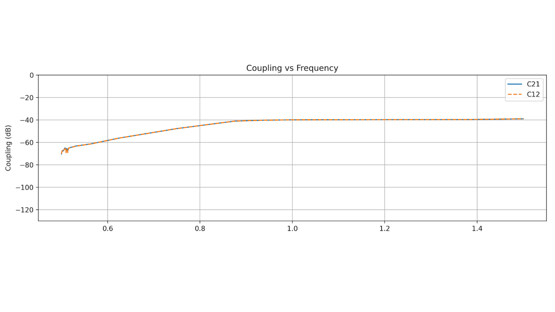
Fig. 3 Coupling between arrays for the 1st case.
# gain vs frequency
ax2.plot(freq_gain, gain_max, label='Installed Gain', color='blue')
ax2.set_xlabel('Frequency (GHz)')
ax2.set_ylabel('Gain (dBi)')
ax2.set_title('Boresight Gain vs Frequency')
ax2.grid(True)
ax2.legend()
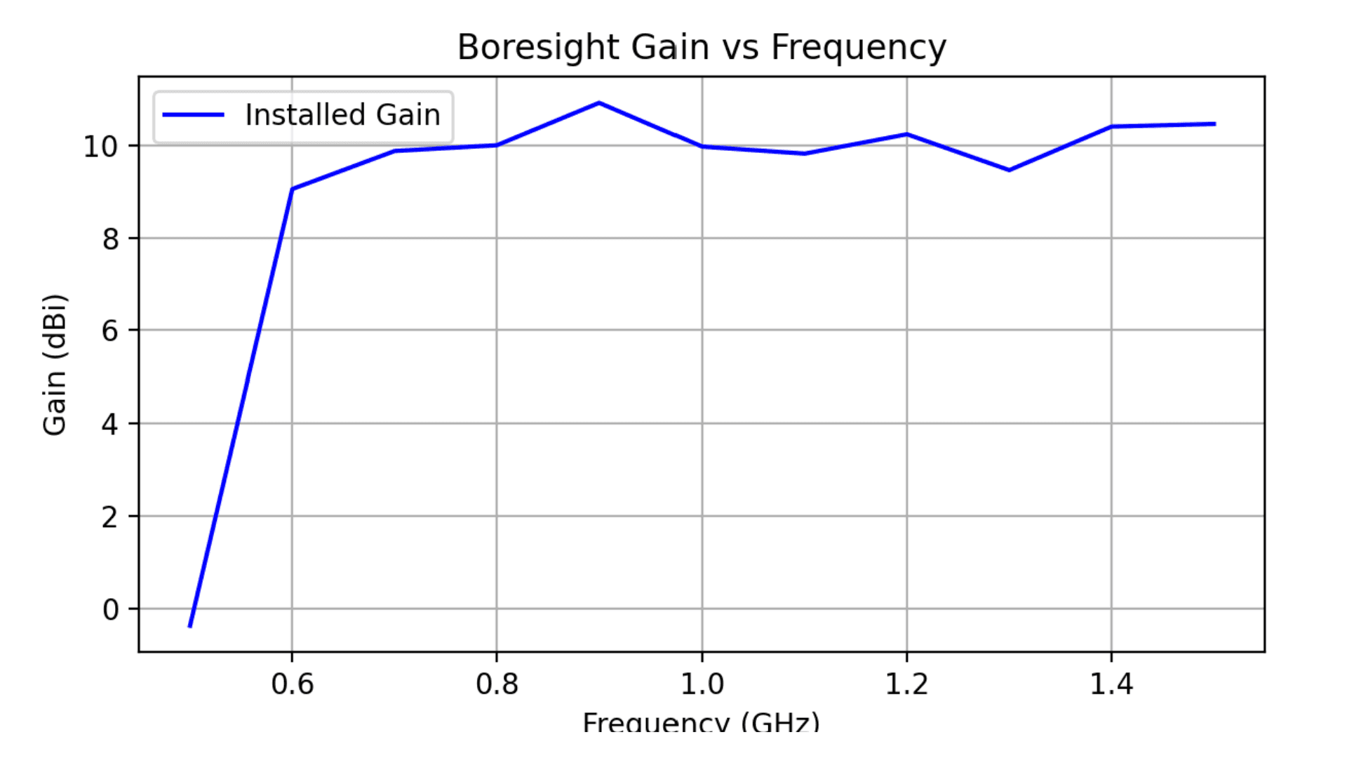
Fig. 4 Boresight gain over frequency for one array
# Polar cut
ax3.plot(np.deg2rad(phi), gain_copol_theta90, color='green', label='Elevation cut (theta=90°)')
ax3.plot(np.deg2rad(theta), gain_copol_phi0, label=f'Azimuth cut', color='red')
ax3.set_title('Cuts')
ax3.set_theta_direction(-1)
ax3.grid(True)
ax3.legend(loc='upper right', bbox_to_anchor=(1.3, 1.1))
plt.tight_layout()

Fig. 5 Elevation and Azimuth cuts: 1st case.
fig3d,ax3d = post_gain.plotPolar3D(gain[:,:,0,freq_idx,1], -20.0,20.0)
fig3d.show()
plt.show()
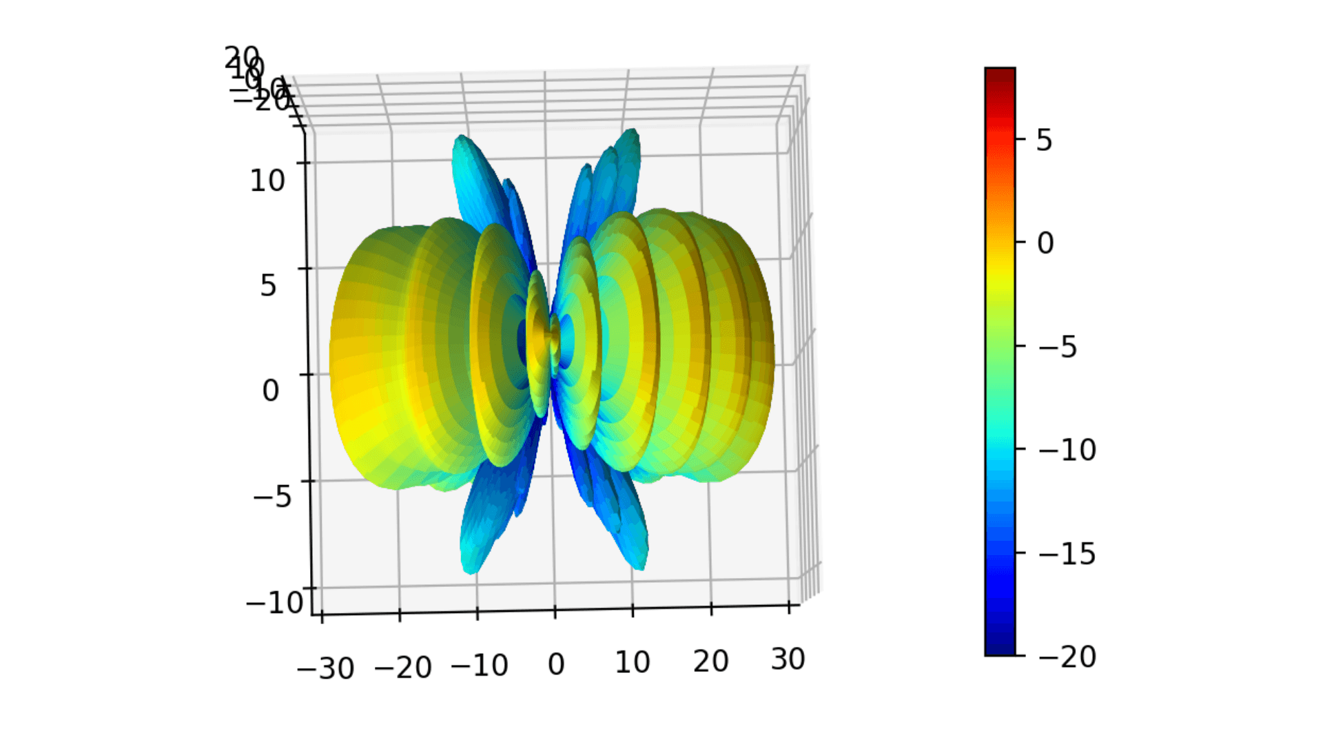
Fig. 6 3D gain pattern: 1st case.
Change phase shifts on both arrays in order to study case #2.
#phase progressions for the two arrays
w1 = progressive_weights(4, phase_deg_per_elem=-30.0) #array1
w2 = progressive_weights(4, phase_deg_per_elem=-30.0) #array2
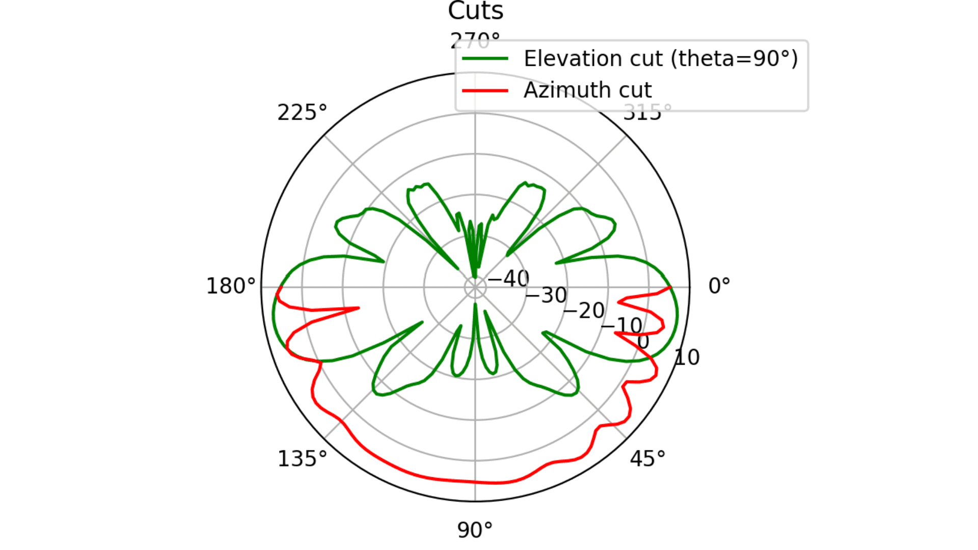
Fig. 7 Elevation and Azimuth cuts: 2nd case.
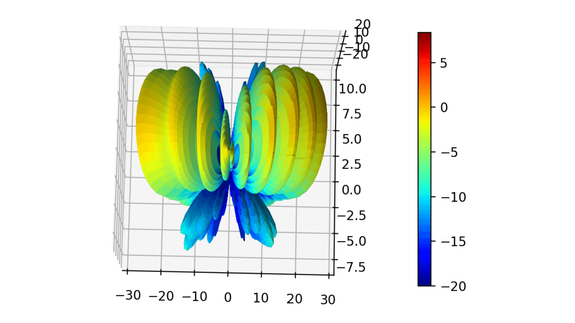
Fig. 8 3D gain pattern: 2nd case.
Change phase shifts on one of the arrays in order to study case #3.
#phase progressions for the two arrays
w1 = progressive_weights(4, phase_deg_per_elem=-30.0) #array1
w2 = progressive_weights(4, phase_deg_per_elem=30.0) #array2
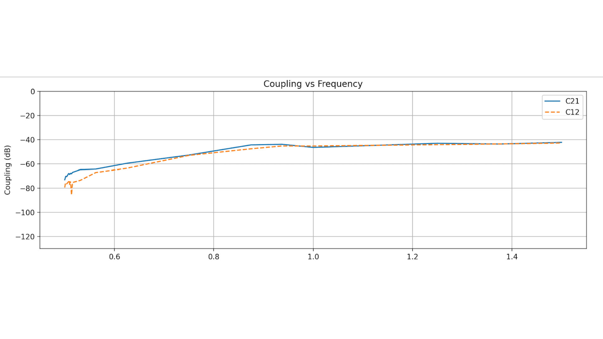
Fig. 9. Coupling between arrays for the 3rd case.
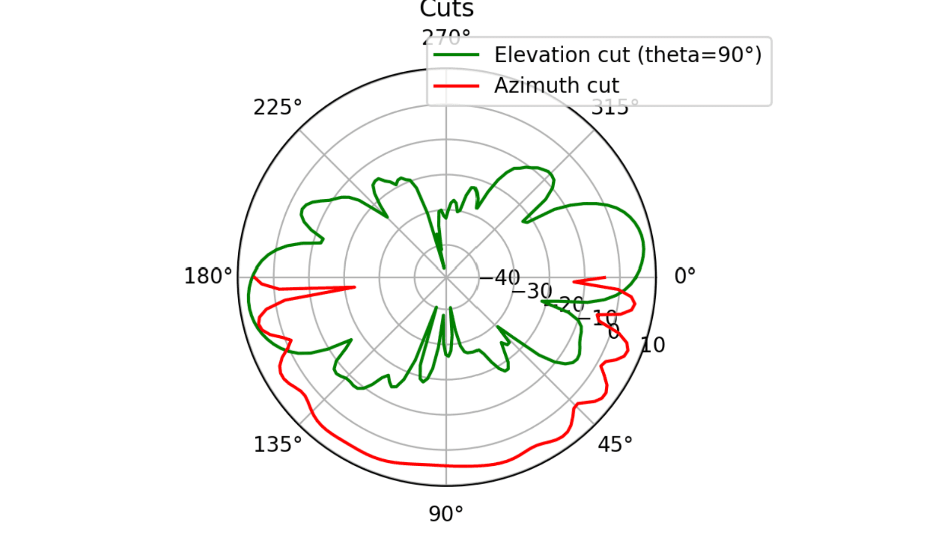
Fig. 10 Elevation and Azimuth cuts: 3rd case.
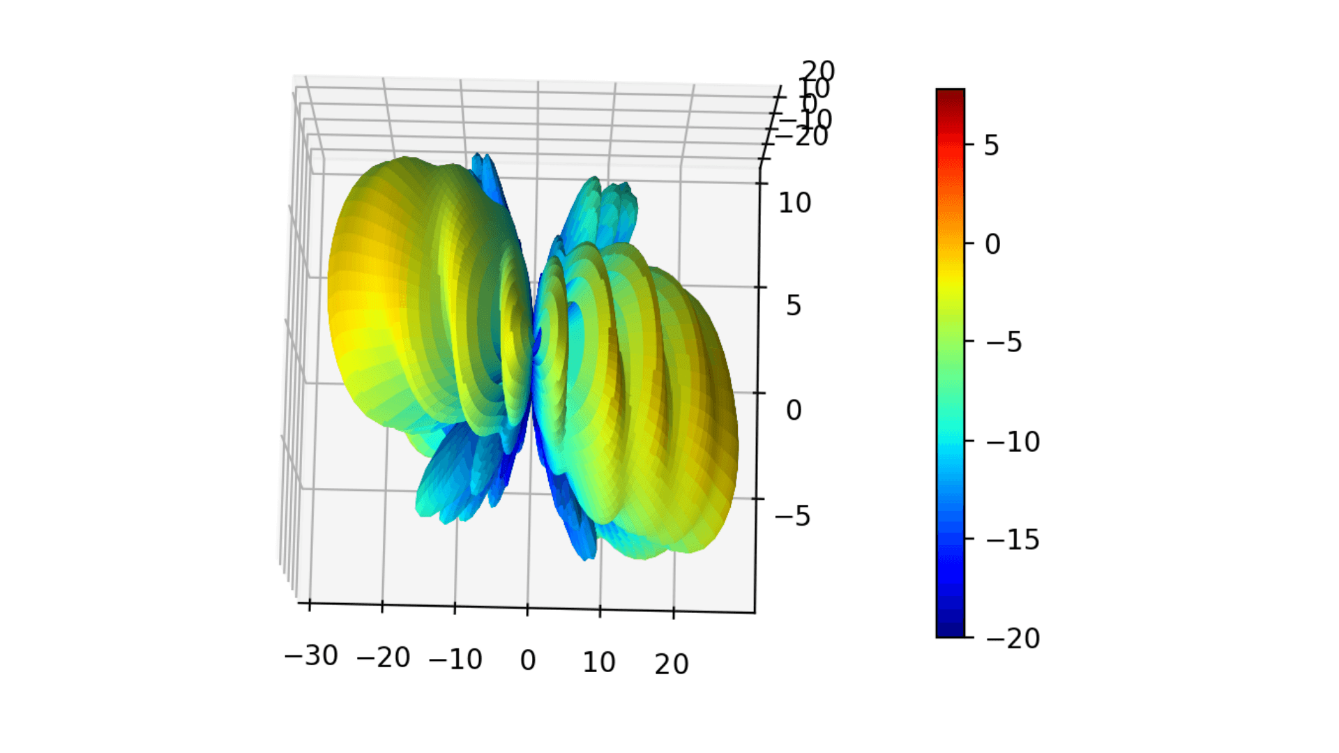
Fig. 11 3D gain pattern: 3rd case.