Antenna Array Installation Simulation Tutorial

This is part 5 of a 6-part tutorial series hosted by experienced antenna engineer Katerina Galitskaya who is documenting her experience learning Nullspace as a new user. Over six tutorials she will progress from simulating a single bow-tie antenna to building full arrays and exploring beamforming techniques, sharing direct comparisons to other full-wave 3D EM simulation tools.

The full video version of this tutorial is available to watch on YouTube.

Problem Statement

This tutorial presents the modeling, simulation, and post-processing of an electrically large problem - a 4-element antenna array installed on a 10-meter telecom tower. The free-space performance of an antenna can differ significantly from its installed performance. Therefore, simulating the antenna array in its actual installation environment is essential for accurate performance evaluation. The final 3D geometry is shown in Figure 1.

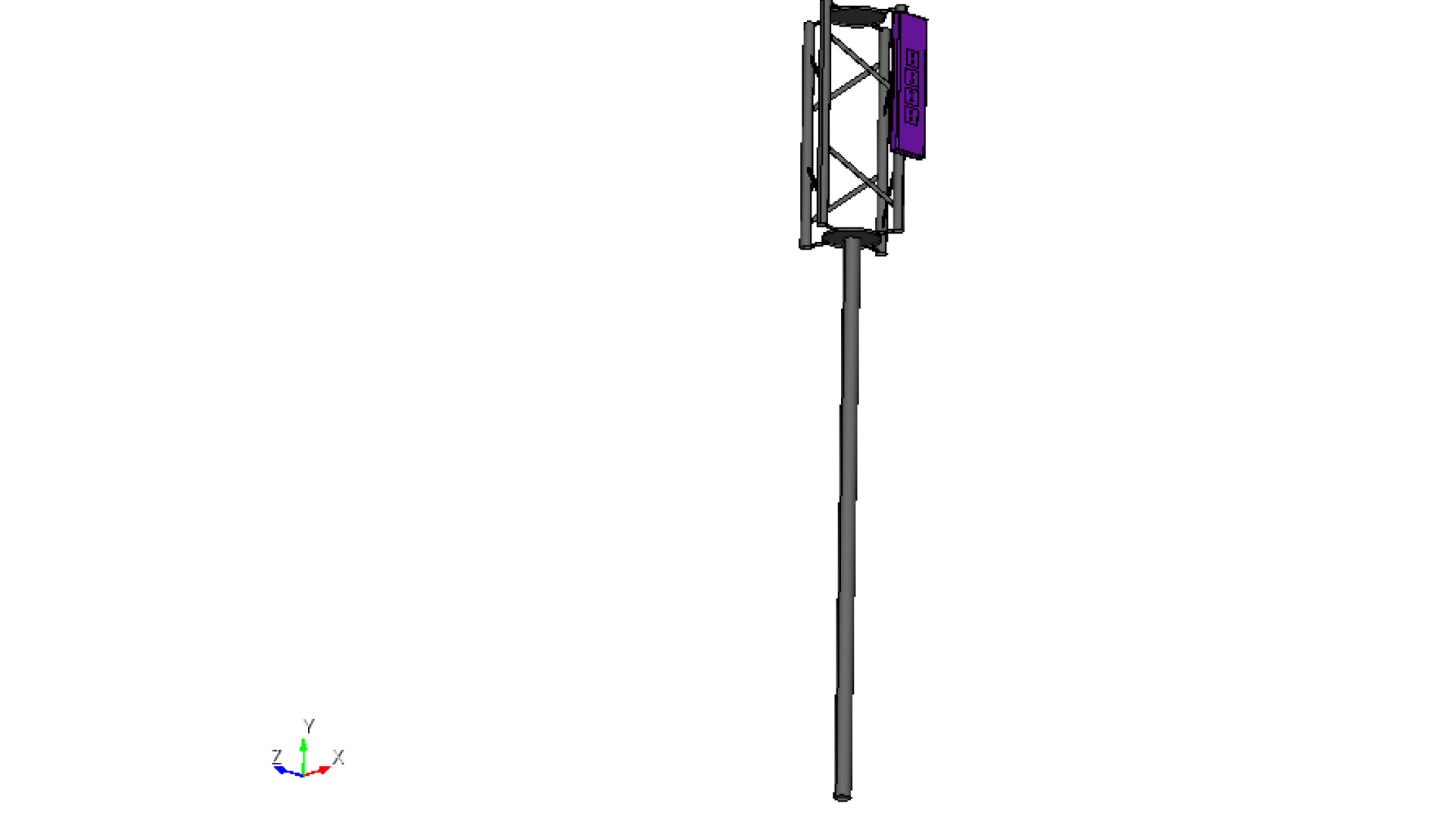
Fig. 1 Integrated antenna array on a tower

Model setup

Preparation: Use the antenna array model from the third tutorial.

Units: CAD model is defined in millimeters, converted to meters during simulation.

Frequency sweep: 0.5–1.5 GHz (51 points).

Radiation data: Dense far‑field grid (2-degree step in theta and phi).

Extracted metrics: Active S-parameters, boresight gain, gain vs. frequency, 2D radiation cuts, and 3D radiation pattern.

CAD Model and Meshing

Begin by opening Prep and setting your working directory to a folder where you plan to complete this example.

Complete the modeling of a 4-element antenna array as described in the previous tutorial.

#{inner_width=1.7}

#{outer_width=30}

#{leng=42}

#{port=1.7}

#{subH=0.767}

#{subW=140}

###substrate geometry

brick x {subW} y {subW} z {subH}

volume 1 rename "substrate"

move Volume substrate z {-subH/2} include_merged 

###ports geometry

create vertex {-port/2} {-port/2} 0 

#{v1 = Id("vertex")}

create vertex {port/2} {-port/2} 0

create vertex {port/2} {0} {port/4}

create vertex {-port/2} {0} {port/4}

create surface vertex {v1} to {v1+3}

#{port_pos = Id("surface")}

surface {port_pos} copy reflect y 

#{port_neg = Id("surface")}

###antenna geometry

create curve location {-outer_width/2} {port/2+leng} 0 location {outer_width/2} {port/2+leng} 0

#{c1 = Id("curve")}

create curve location {-outer_width/2} {port/2+leng} 0 location {-inner_width/2} {port/2} 0

create curve location {outer_width/2} {port/2+leng} 0 location {inner_width/2} {port/2} 0

create curve location {-inner_width/2} {port/2} 0 location {inner_width/2} {port/2} 0

create surface curve {c1} to {c1+3}

#{dipole_top = Id("surface")}

surface {dipole_top} copy reflect y nomesh 

#{dipole_bot = Id("surface")}

project surface {port_pos} {port_neg} onto surface 1 imprint

project surface {port_pos} {port_neg} {dipole_top} {dipole_bot} onto surface 2 imprint

###ground plane

create surface rectangle width 300 zplane 

#{GND = Id("surface")}

#{gnd_H=70}

move Volume 6 z {-gnd_H} include_merged preview 

move Volume 6 z {-gnd_H} include_merged 

###4-element array creation

Volume 1 2 3 4 5 6 copy move x 0 y 170 z 0 repeat 3 group_results 

unite surface {GND} 36 53 70 

#{GND = Id("surface")}

import step "radome.step" heal group "radome" ### importing step file of the radome

#{radome = Id("volume")} ### getting a variable for the radome volume ID

move volume {radome} y -170 include_merged #### center the radome to array geometry

rotate Volume all angle 90 about Y include_merged preview 

rotate Volume all angle 90 about Y include_merged 

Import the STEP file for the telecom tower. Ensure that the file path is correctly specified. 

###tower import

import step "TelecomMast_simplified.step" heal group "Tower" 

#{tower = Id("volume")}

Position the tower so the antenna array is mounted on one of the poles.

move volume {tower} x -580 y -11000 z 130 include_merged

Simplify the mast geometry by removing unnecessary small features and surfaces. Some simplifications require decomposing a volume into simpler parts using the webcut function.

### Remove small features and surfaces from tower model

remove surface 181, 200 connected_sets

remove surface 88, 170, 199 connected_sets

select surface 183 include similar

remove surface 179, 183 connected_sets

select surface 198 118 203 include similar

remove surface 118, 198, 203, 204 connected_sets

remove surface 168

remove surface 182, 201 connected_sets

remove surface 154, 202 connected_sets

remove surface 180

remove surface 184

select surface 143 207 include similar

remove surface 143, 151, 206, 207 connected_sets

remove surface 187

remove surface 91, 92, 126 connected_sets

remove surface 122, 150, 158 connected_sets

remove surface 99, 134, 167 connected_sets

webcut volume 26 with sheet extended from surface 146 

webcut volume 27 with sheet extended from surface 205 

delete volume 27

remove surface 123, 127, 128 connected_sets

imprint all

merge all

Materials & Voltage Sources

Use the material.py script to define the material library. Besides PEC, this model uses FR-4 and glass fiber. Open the Nullspace EM environment and load the material.py file before assigning materials.

from nsem import *

ml=MaterialLibrary()

ml.add_material(Material('FR-4', 'green', MaterialProperty('constant',real=4.4, losstan=0.02), MaterialProperty('constant',real=1.0, imag=0.0)))

ml.add_material(Material('glassfiber', 'grey', MaterialProperty('constant',real=4.7, losstan=0.09), MaterialProperty('constant',real=1.0, imag=0.0)))

ml.save('materials')

Assign materials and define four voltage sources. Ensure consistent assignment of positive and negative terminals across all ports.

nsem load material library 'materials.h5'

nsem assign volume substrate material 'FR-4' ###the original substrate 

nsem assign volume 7 13 19 material 'FR-4' ###the 3 copies

nsem assign volume {radome} material 'glassfiber' ### glass fiber material to the radome

nsem assign surface {dipole_top} {dipole_bot} material 'PEC' ###the original antenna

nsem assign surface 34 35 36 51 52 53 68 69 70 material 'PEC' ###the 3 copies

nsem assign surface {GND} material 'PEC' ### ground plane material

nsem assign volume {tower} 28 material 'PEC' ### telecom tower material

nsem voltage source 'port_001' pos surface {port_pos} neg surface {port_neg} impedance 50 

nsem voltage source 'port_002' pos surface 32 neg surface 33 impedance 50

nsem voltage source 'port_003' pos surface 49 neg surface 50 impedance 50

nsem voltage source 'port_004' pos surface 66 neg surface 67 impedance 50

Meshing

Repeat the meshing as shown in the previous tutorial. Use lambda/10 meshing for the telecom mast. 

###meshing

surface all scheme pave

#{mesh=0.3/1*1000/10}

###port meshing

group 'feed' add surface {port_pos} {port_neg} 32 33 49 50 66 67

curve common_to surface in feed interval 1

mesh surface in feed

###antenna meshing

surface {dipole_top} {dipole_bot} 34 35 51 52 68 69 size {mesh/4}

mesh surface {dipole_top} {dipole_bot} 34 35 51 52 68 69

surface 14 16 17 18 size {mesh/4}

mesh surface 14 16 17 18

surface {GND} size {mesh/1.5}

mesh surface {GND}

surface not is_meshed in volume 1 7 13 19 size {mesh/4}

mesh surface not is_meshed in volume 1 7 13 19

###radome meshing

surface not is_meshed in volume {radome} size {mesh}

mesh surface not is_meshed in volume {radome}

### telecom tower meshing

###small features 

surface 102 size 20

mesh surface 102 

surface 224 size 20

mesh surface 224 

###rest of the tower meshing

surface not is_meshed in volume {tower} size {mesh}

mesh surface not is_meshed in volume {tower}

surface not is_meshed in volume 28 size {mesh}

mesh surface not is_meshed in volume 28

Generate a mesh quality plot to identify potential problem areas.

quality surface all shape global draw mesh

save cub5 "tower_array.cub5" overwrite journal

Fig. 2 Model with the mesh quality plotted.

Simulation Setup

Create a simulation.py file to configure the simulation parameters. Since the structure is electrically large, use the compression solver, which performs matrix compression and leverages near- and far-field coupling to efficiently represent the system.

from nsem import *

import numpy as np

config = 'tower_array'

model = Configuration(f'{config}_sim') #configure simulation name

model.set_cub5_filename(f'{config}.cub5') #load the mesh file

model.set_order(1) #set basis order, default is 1

model.set_model_scale(0.001) #convertion to mm

model.set_frequencies(freq_beg=0.5, freq_end=1.5) #set frequency sweep from 0.5 to 1.5 GHz

model.set_solve_type(solver='COMPRESS') #change the solver type

model.save()

report = Report(f'{config}_report', f'{config}_sim') #create a report object

report.set_frequencies(np.linspace(0.5, 1.5, 11))

step = 2 #set the step for theta and phi angles 

theta_scan = np.linspace(0, 180, int(180/step+1)) #theta angles from 0 to 180 degrees

phi_scan = np.linspace(0, 360, int(360/step)) #phi angles from 0 to 360 degrees

report.request_far_fields_grid(theta_scan, phi_scan) #request far-field data

report.save() #save the report configuration

model.run() #run the simulation

report.run() #run the report generation

Post-Processing

Create postprocessing.py to extract simulation data and visualize results.

import matplotlib.pyplot as plt

import numpy as np

from nsem.postprocessing import *  

from scipy.interpolate import CubicSpline

config = 'tower_array'

post = PostProcess(f'{config}_sim')  # create a post-processing object for the simulation

freq = post.get_frequencies()  # get the frequencies

freq = np.linspace(np.min(freq), np.max(freq), 501)  # create a frequency array for evaluation

w = [1.0, 1.0, 1.0, 1.0] # excitation of each port

active_s = post.get_active_s_parameters(freq_evaluate=freq,weights=w)

active_s11 = dB20(np.squeeze(active_s[0, :]))

active_s22 = dB20(np.squeeze(active_s[1, :]))

active_s33 = dB20(np.squeeze(active_s[2, :]))

active_s44 = dB20(np.squeeze(active_s[3, :]))

#plots

fig = plt.figure(figsize=(18, 6))

ax1 = plt.subplot(1, 3, 1)

ax2 = plt.subplot(1, 3, 2)

ax3 = plt.subplot(1, 3, 3, polar=True)

# active S-parameters

ax1.plot(freq, active_s11, label='active S11', color='blue')

ax1.plot(freq, active_s22, label='active S22', color='orange')

ax1.plot(freq, active_s33, label='active S33', color='green')

ax1.plot(freq, active_s44, label='active S44', color='red')

ax1.set_xlabel('Frequency (GHz)')

ax1.set_ylabel('S11 (dB)')

ax1.set_title('Active S-parameters')

ax1.grid(True)

ax1.legend()

Fig. 3 Active S11 for each port

post = PostProcess(f'{config}_report')  # create a post-processing object for the report

freq = post.get_frequencies()

theta = post.get_obs_theta()

phi = post.get_obs_phi()

gain = post.get_gain('spherical',weights=w)  #get gain with specified amplitude/phase distribution

theta_idx,_ = post.get_nearest(theta, 0.0)

phi0_idx,_  = post.get_nearest(phi, 0.0)

phi90_idx,_  = post.get_nearest(phi, 90.0)

theta90_idx,_ = post.get_nearest(theta, 90.0)

theta0_idx,_ = post.get_nearest(theta, 0.0)

freq_idx,_ = post.get_nearest(freq, 1.0)

gain_0 = gain[phi0_idx, theta90_idx, 0, freq_idx, 1]

print(f"Boresight gain (dBi): {gain_0:.2f}")

gain_copol_phi0  = gain[phi0_idx, :, 0, freq_idx,1]

gain_copol_phi90 = gain[phi90_idx, :, 0, freq_idx, 0]

gain_xpol_phi0   = gain[phi0_idx, :, 0, freq_idx, 0]

gain_xpol_phi90  = gain[phi90_idx, :, 0, freq_idx, 1]  

gain_copol_theta90 = gain[:, theta90_idx, 0, freq_idx, 1]   

gain_xpol_theta90  = gain[:, theta90_idx, 0, freq_idx, 0]

#Gain plot interpolation

gain_max = np.squeeze(gain[phi0_idx, theta90_idx, 0, :, 1])

x = np.asarray(freq).ravel()

y = np.asarray(gain_max).ravel()

x_unique, idx = np.unique(x, return_index=True)

y_unique = y[idx]

cs = CubicSpline(x_unique, y_unique, bc_type='natural', extrapolate=False)

x_dense = np.linspace(x_unique[0], x_unique[-1], 501)

y_dense = cs(x_dense)

# Gain vs frequency 

ax2.plot(x_dense, y_dense, label='Gain with radome', color='blue')

ax2.set_xlabel('Frequency (GHz)')

ax2.set_ylabel('Gain (dBi)')

ax2.set_title('Boresight Gain vs Frequency')

ax2.grid(True)

ax2.legend()

Fig. 4 Boresight gain over frequency

# Elevation and azimuth cuts

ax3.plot(np.deg2rad(phi), gain_copol_theta90, label=f'Co-pol theta=90°', color='green')

ax3.plot(np.deg2rad(theta), gain_copol_phi0, label=f'Azimuth cut', color='red')

ax3.set_xlabel('phi (deg)')

ax3.set_ylabel('Gain (dBi)')

ax3.set_title('Cuts')

ax3.grid(True)

ax3.legend()

fig.tight_layout()

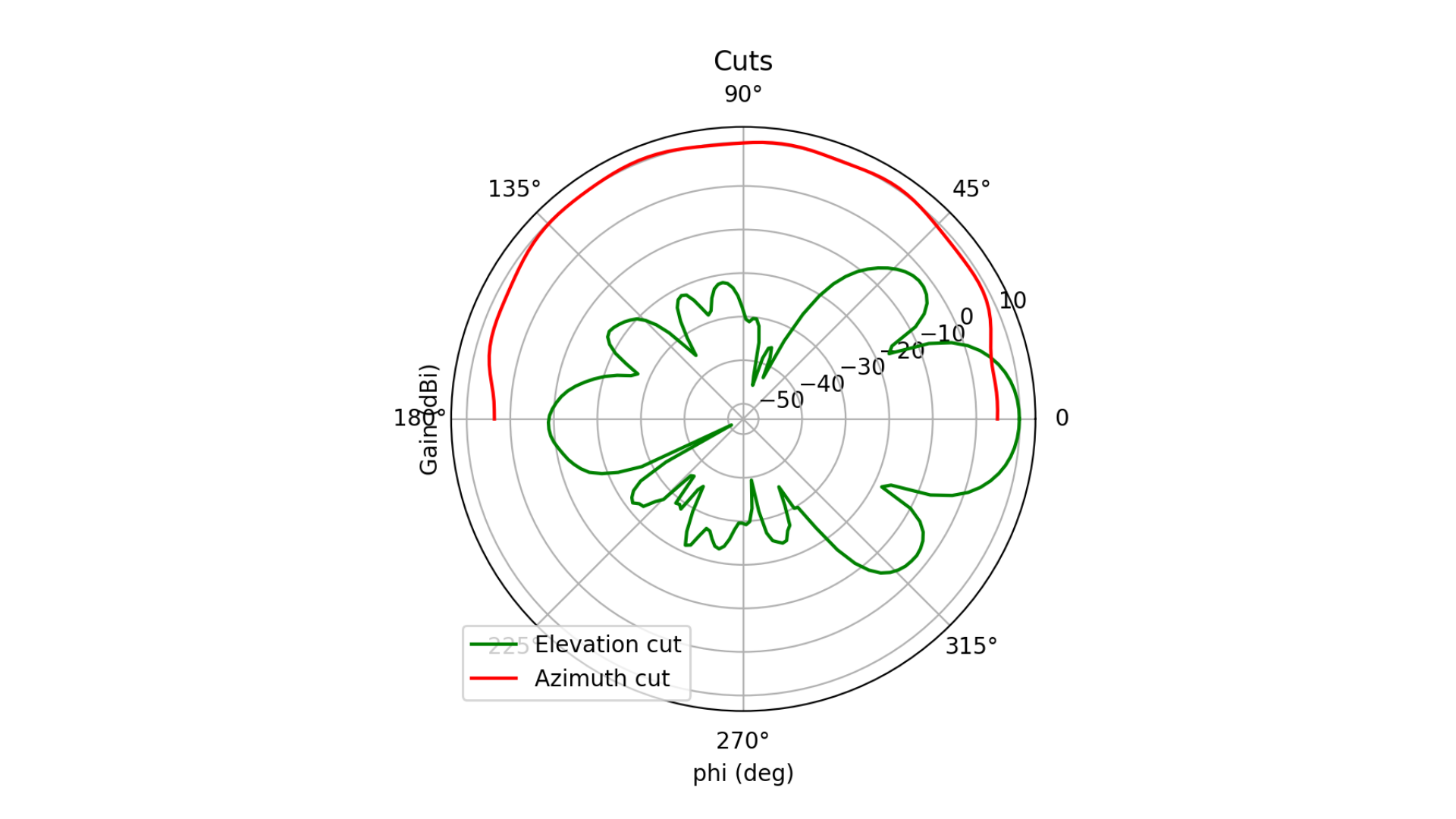
Fig. 5 Elevation and Azimuth cuts

#3D radiation pattern

fig3d,ax3d = post.plotPolar3D(gain[:,:,0,freq_idx,1], -20.0,20.0)

fig3d.show()

plt.show()

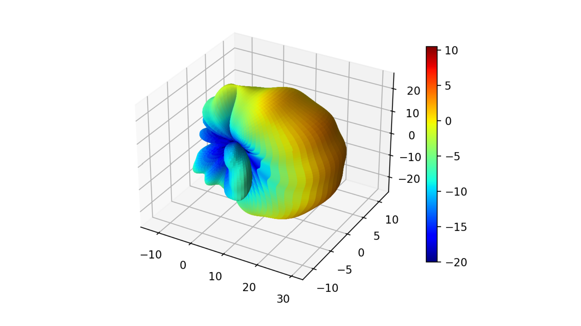
Fig. 6 3D gain pattern